
7. Loading data into python
In this section, we are taking a look at loading data into python. We will talk about some general data formats and discuss strategies to get data out of e.g. instrument control software and into your evaluation scripts.
We will look at the following file types in this chapter:
tabulated data in text files
MS Excel and LibreOffice Calc
7.1. tabulated data in text files (“CSV”)
The category of tabulated data in text files is pretty loosely defined, and there are not really any standards for it. I am going to use the term “CSV” here pretty loosely for any type of human readable tabulated data, even though it actually is an abbreviation for one specific type of format of “comma separated values”.
In general CSVs consist of rows of data encoded in a human readable format (e.g. ASCII, unicode). There is some delimiter character that separates rows and a new line to separate columns. Delimiter characters are typically ,, but ;, spaces or tabs are also commonly used. In some files the first row describes the data contained in each column. Sometimes, there is a header that describes the contents of the file (e.g. measurement parameters, date, time and so on).
To import CSVs into python, there are several functions. We will focus on numpy.genfromtxt and pandas.read_csv here. The main difference here is, that numpy.genfromtxt outputs a numpy array, while pandas.read_csv outputs a pandas DataFrame. You can use genfromtxt for data that is mostly numerical, whereas read_csv works well for mixed data, but is potentially less performant.
When importing a CSV, we need to first check the following info:
What data do we expect?
Which delimiter is used?
What is the line number of the first table row?
Are there commments or a header?
Is the number format “weird”? (E.g.
,instead of.for decimal seperator)Do rows contain text data?
The best way to check these is to use a text editor. Unfortunately, the default editor in Windows “Notepad” is really bad. Instead, you can download “Notepad ++” or “Programmer’s Notebook” or use Jupyter to open text files. Just click on the file name in the Jupyter file browser.
When using Notepad ++, you can turn on showing white space in the “View>Show Symbol>White Space and TAB” menu.
Let’s have a look at an example for such a CSV file, “data/64-17-5-IR.csv”. Since we are not sure what the file looks like, we have to check using an editor. Here are the first few lines of the file as they appear in Notepad++:

1. What data do we expect?
This file contains an infrared spectrum in a column shape. The first column contains the wavenumber axis, the second column contains the absorption values.
2. What is the delimiter?
The orange arrows are how the program shows TABs when show white spaces is enabled. So our delimiters are TABs.
3. What is the line number of the first table row?
From the screen shot above, we also see that the first line contains a header. The data starts in the second line.
4. Are there commments or a header?
There are no comments but the first line contains column headers.
5. Is the number format “weird”?
No, there is nothing unexpected in the number format.
6. Do rows contain text data?
No.
Now, we are ready to import the file. Since the delimiter here is a white space character (TAB), we don’t have to specify it in the call to genfromtxt. That is covered by the default arguments. If we wanted to specify TAB explicitly, we would use the optional argument delimiter='\t'.
The row containing data is in the second line of the file, hence we pass the optional argument skip_header=1. The number format consists of integers and there is no text data:
import numpy as np

loaded_data = np.genfromtxt(fname="data/64-17-5-IR.csv", skip_header=1)
loaded_data
array([[4.500e+02, 1.670e-02],
       [4.540e+02, 4.506e-02],
       [4.580e+02, 5.056e-02],
       ...,
       [3.958e+03, 5.493e-03],
       [3.962e+03, 5.156e-03],
       [3.966e+03, 4.260e-03]])
The returned array has the same shape as the table in the CSV file. We can get individual entries using indexing:
loaded_data[1,1]
0.04506
We can also adress rows using either just the first index
loaded_data[0]
array([4.50e+02, 1.67e-02])
or the first index and a colon for the second index:
loaded_data[0,:]
array([4.50e+02, 1.67e-02])
We can also select columns using the colon for the first index and a number for the second index
loaded_data[:,0]
array([ 450.,  454.,  458.,  462.,  466.,  470.,  474.,  478.,  482.,
        486.,  490.,  494.,  498.,  502.,  506.,  510.,  514.,  518.,
        522.,  526.,  530.,  534.,  538.,  542.,  546.,  550.,  554.,
        558.,  562.,  566.,  570.,  574.,  578.,  582.,  586.,  590.,
        594.,  598.,  602.,  606.,  610.,  614.,  618.,  622.,  626.,
        630.,  634.,  638.,  642.,  646.,  650.,  654.,  658.,  662.,
        666.,  670.,  674.,  678.,  682.,  686.,  690.,  694.,  698.,
        702.,  706.,  710.,  714.,  718.,  722.,  726.,  730.,  734.,
        738.,  742.,  746.,  750.,  754.,  758.,  762.,  766.,  770.,
        774.,  778.,  782.,  786.,  790.,  794.,  798.,  802.,  806.,
        810.,  814.,  818.,  822.,  826.,  830.,  834.,  838.,  842.,
        846.,  850.,  854.,  858.,  862.,  866.,  870.,  874.,  878.,
        882.,  886.,  890.,  894.,  898.,  902.,  906.,  910.,  914.,
        918.,  922.,  926.,  930.,  934.,  938.,  942.,  946.,  950.,
        954.,  958.,  962.,  966.,  970.,  974.,  978.,  982.,  986.,
        990.,  994.,  998., 1002., 1006., 1010., 1014., 1018., 1022.,
       1026., 1030., 1034., 1038., 1042., 1046., 1050., 1054., 1058.,
       1062., 1066., 1070., 1074., 1078., 1082., 1086., 1090., 1094.,
       1098., 1102., 1106., 1110., 1114., 1118., 1122., 1126., 1130.,
       1134., 1138., 1142., 1146., 1150., 1154., 1158., 1162., 1166.,
       1170., 1174., 1178., 1182., 1186., 1190., 1194., 1198., 1202.,
       1206., 1210., 1214., 1218., 1222., 1226., 1230., 1234., 1238.,
       1242., 1246., 1250., 1254., 1258., 1262., 1266., 1270., 1274.,
       1278., 1282., 1286., 1290., 1294., 1298., 1302., 1306., 1310.,
       1314., 1318., 1322., 1326., 1330., 1334., 1338., 1342., 1346.,
       1350., 1354., 1358., 1362., 1366., 1370., 1374., 1378., 1382.,
       1386., 1390., 1394., 1398., 1402., 1406., 1410., 1414., 1418.,
       1422., 1426., 1430., 1434., 1438., 1442., 1446., 1450., 1454.,
       1458., 1462., 1466., 1470., 1474., 1478., 1482., 1486., 1490.,
       1494., 1498., 1502., 1506., 1510., 1514., 1518., 1522., 1526.,
       1530., 1534., 1538., 1542., 1546., 1550., 1554., 1558., 1562.,
       1566., 1570., 1574., 1578., 1582., 1586., 1590., 1594., 1598.,
       1602., 1606., 1610., 1614., 1618., 1622., 1626., 1630., 1634.,
       1638., 1642., 1646., 1650., 1654., 1658., 1662., 1666., 1670.,
       1674., 1678., 1682., 1686., 1690., 1694., 1698., 1702., 1706.,
       1710., 1714., 1718., 1722., 1726., 1730., 1734., 1738., 1742.,
       1746., 1750., 1754., 1758., 1762., 1766., 1770., 1774., 1778.,
       1782., 1786., 1790., 1794., 1798., 1802., 1806., 1810., 1814.,
       1818., 1822., 1826., 1830., 1834., 1838., 1842., 1846., 1850.,
       1854., 1858., 1862., 1866., 1870., 1874., 1878., 1882., 1886.,
       1890., 1894., 1898., 1902., 1906., 1910., 1914., 1918., 1922.,
       1926., 1930., 1934., 1938., 1942., 1946., 1950., 1954., 1958.,
       1962., 1966., 1970., 1974., 1978., 1982., 1986., 1990., 1994.,
       1998., 2002., 2006., 2010., 2014., 2018., 2022., 2026., 2030.,
       2034., 2038., 2042., 2046., 2050., 2054., 2058., 2062., 2066.,
       2070., 2074., 2078., 2082., 2086., 2090., 2094., 2098., 2102.,
       2106., 2110., 2114., 2118., 2122., 2126., 2130., 2134., 2138.,
       2142., 2146., 2150., 2154., 2158., 2162., 2166., 2170., 2174.,
       2178., 2182., 2186., 2190., 2194., 2198., 2202., 2206., 2210.,
       2214., 2218., 2222., 2226., 2230., 2234., 2238., 2242., 2246.,
       2250., 2254., 2258., 2262., 2266., 2270., 2274., 2278., 2282.,
       2286., 2290., 2294., 2298., 2302., 2306., 2310., 2314., 2318.,
       2322., 2326., 2330., 2334., 2338., 2342., 2346., 2350., 2354.,
       2358., 2362., 2366., 2370., 2374., 2378., 2382., 2386., 2390.,
       2394., 2398., 2402., 2406., 2410., 2414., 2418., 2422., 2426.,
       2430., 2434., 2438., 2442., 2446., 2450., 2454., 2458., 2462.,
       2466., 2470., 2474., 2478., 2482., 2486., 2490., 2494., 2498.,
       2502., 2506., 2510., 2514., 2518., 2522., 2526., 2530., 2534.,
       2538., 2542., 2546., 2550., 2554., 2558., 2562., 2566., 2570.,
       2574., 2578., 2582., 2586., 2590., 2594., 2598., 2602., 2606.,
       2610., 2614., 2618., 2622., 2626., 2630., 2634., 2638., 2642.,
       2646., 2650., 2654., 2658., 2662., 2666., 2670., 2674., 2678.,
       2682., 2686., 2690., 2694., 2698., 2702., 2706., 2710., 2714.,
       2718., 2722., 2726., 2730., 2734., 2738., 2742., 2746., 2750.,
       2754., 2758., 2762., 2766., 2770., 2774., 2778., 2782., 2786.,
       2790., 2794., 2798., 2802., 2806., 2810., 2814., 2818., 2822.,
       2826., 2830., 2834., 2838., 2842., 2846., 2850., 2854., 2858.,
       2862., 2866., 2870., 2874., 2878., 2882., 2886., 2890., 2894.,
       2898., 2902., 2906., 2910., 2914., 2918., 2922., 2926., 2930.,
       2934., 2938., 2942., 2946., 2950., 2954., 2958., 2962., 2966.,
       2970., 2974., 2978., 2982., 2986., 2990., 2994., 2998., 3002.,
       3006., 3010., 3014., 3018., 3022., 3026., 3030., 3034., 3038.,
       3042., 3046., 3050., 3054., 3058., 3062., 3066., 3070., 3074.,
       3078., 3082., 3086., 3090., 3094., 3098., 3102., 3106., 3110.,
       3114., 3118., 3122., 3126., 3130., 3134., 3138., 3142., 3146.,
       3150., 3154., 3158., 3162., 3166., 3170., 3174., 3178., 3182.,
       3186., 3190., 3194., 3198., 3202., 3206., 3210., 3214., 3218.,
       3222., 3226., 3230., 3234., 3238., 3242., 3246., 3250., 3254.,
       3258., 3262., 3266., 3270., 3274., 3278., 3282., 3286., 3290.,
       3294., 3298., 3302., 3306., 3310., 3314., 3318., 3322., 3326.,
       3330., 3334., 3338., 3342., 3346., 3350., 3354., 3358., 3362.,
       3366., 3370., 3374., 3378., 3382., 3386., 3390., 3394., 3398.,
       3402., 3406., 3410., 3414., 3418., 3422., 3426., 3430., 3434.,
       3438., 3442., 3446., 3450., 3454., 3458., 3462., 3466., 3470.,
       3474., 3478., 3482., 3486., 3490., 3494., 3498., 3502., 3506.,
       3510., 3514., 3518., 3522., 3526., 3530., 3534., 3538., 3542.,
       3546., 3550., 3554., 3558., 3562., 3566., 3570., 3574., 3578.,
       3582., 3586., 3590., 3594., 3598., 3602., 3606., 3610., 3614.,
       3618., 3622., 3626., 3630., 3634., 3638., 3642., 3646., 3650.,
       3654., 3658., 3662., 3666., 3670., 3674., 3678., 3682., 3686.,
       3690., 3694., 3698., 3702., 3706., 3710., 3714., 3718., 3722.,
       3726., 3730., 3734., 3738., 3742., 3746., 3750., 3754., 3758.,
       3762., 3766., 3770., 3774., 3778., 3782., 3786., 3790., 3794.,
       3798., 3802., 3806., 3810., 3814., 3818., 3822., 3826., 3830.,
       3834., 3838., 3842., 3846., 3850., 3854., 3858., 3862., 3866.,
       3870., 3874., 3878., 3882., 3886., 3890., 3894., 3898., 3902.,
       3906., 3910., 3914., 3918., 3922., 3926., 3930., 3934., 3938.,
       3942., 3946., 3950., 3954., 3958., 3962., 3966.])
If we are going to look at column wise data most of the time, it is shorter to use the unpack=True optional argument. This loads the data and then transposes it:
loaded_data = np.genfromtxt(fname="data/64-17-5-IR.csv",
                            skip_header=1,
                            unpack=True)
loaded_data
array([[4.500e+02, 4.540e+02, 4.580e+02, ..., 3.958e+03, 3.962e+03,
        3.966e+03],
       [1.670e-02, 4.506e-02, 5.056e-02, ..., 5.493e-03, 5.156e-03,
        4.260e-03]])
Now we can select columns in the file using the first index:
loaded_data[0]
array([ 450.,  454.,  458.,  462.,  466.,  470.,  474.,  478.,  482.,
        486.,  490.,  494.,  498.,  502.,  506.,  510.,  514.,  518.,
        522.,  526.,  530.,  534.,  538.,  542.,  546.,  550.,  554.,
        558.,  562.,  566.,  570.,  574.,  578.,  582.,  586.,  590.,
        594.,  598.,  602.,  606.,  610.,  614.,  618.,  622.,  626.,
        630.,  634.,  638.,  642.,  646.,  650.,  654.,  658.,  662.,
        666.,  670.,  674.,  678.,  682.,  686.,  690.,  694.,  698.,
        702.,  706.,  710.,  714.,  718.,  722.,  726.,  730.,  734.,
        738.,  742.,  746.,  750.,  754.,  758.,  762.,  766.,  770.,
        774.,  778.,  782.,  786.,  790.,  794.,  798.,  802.,  806.,
        810.,  814.,  818.,  822.,  826.,  830.,  834.,  838.,  842.,
        846.,  850.,  854.,  858.,  862.,  866.,  870.,  874.,  878.,
        882.,  886.,  890.,  894.,  898.,  902.,  906.,  910.,  914.,
        918.,  922.,  926.,  930.,  934.,  938.,  942.,  946.,  950.,
        954.,  958.,  962.,  966.,  970.,  974.,  978.,  982.,  986.,
        990.,  994.,  998., 1002., 1006., 1010., 1014., 1018., 1022.,
       1026., 1030., 1034., 1038., 1042., 1046., 1050., 1054., 1058.,
       1062., 1066., 1070., 1074., 1078., 1082., 1086., 1090., 1094.,
       1098., 1102., 1106., 1110., 1114., 1118., 1122., 1126., 1130.,
       1134., 1138., 1142., 1146., 1150., 1154., 1158., 1162., 1166.,
       1170., 1174., 1178., 1182., 1186., 1190., 1194., 1198., 1202.,
       1206., 1210., 1214., 1218., 1222., 1226., 1230., 1234., 1238.,
       1242., 1246., 1250., 1254., 1258., 1262., 1266., 1270., 1274.,
       1278., 1282., 1286., 1290., 1294., 1298., 1302., 1306., 1310.,
       1314., 1318., 1322., 1326., 1330., 1334., 1338., 1342., 1346.,
       1350., 1354., 1358., 1362., 1366., 1370., 1374., 1378., 1382.,
       1386., 1390., 1394., 1398., 1402., 1406., 1410., 1414., 1418.,
       1422., 1426., 1430., 1434., 1438., 1442., 1446., 1450., 1454.,
       1458., 1462., 1466., 1470., 1474., 1478., 1482., 1486., 1490.,
       1494., 1498., 1502., 1506., 1510., 1514., 1518., 1522., 1526.,
       1530., 1534., 1538., 1542., 1546., 1550., 1554., 1558., 1562.,
       1566., 1570., 1574., 1578., 1582., 1586., 1590., 1594., 1598.,
       1602., 1606., 1610., 1614., 1618., 1622., 1626., 1630., 1634.,
       1638., 1642., 1646., 1650., 1654., 1658., 1662., 1666., 1670.,
       1674., 1678., 1682., 1686., 1690., 1694., 1698., 1702., 1706.,
       1710., 1714., 1718., 1722., 1726., 1730., 1734., 1738., 1742.,
       1746., 1750., 1754., 1758., 1762., 1766., 1770., 1774., 1778.,
       1782., 1786., 1790., 1794., 1798., 1802., 1806., 1810., 1814.,
       1818., 1822., 1826., 1830., 1834., 1838., 1842., 1846., 1850.,
       1854., 1858., 1862., 1866., 1870., 1874., 1878., 1882., 1886.,
       1890., 1894., 1898., 1902., 1906., 1910., 1914., 1918., 1922.,
       1926., 1930., 1934., 1938., 1942., 1946., 1950., 1954., 1958.,
       1962., 1966., 1970., 1974., 1978., 1982., 1986., 1990., 1994.,
       1998., 2002., 2006., 2010., 2014., 2018., 2022., 2026., 2030.,
       2034., 2038., 2042., 2046., 2050., 2054., 2058., 2062., 2066.,
       2070., 2074., 2078., 2082., 2086., 2090., 2094., 2098., 2102.,
       2106., 2110., 2114., 2118., 2122., 2126., 2130., 2134., 2138.,
       2142., 2146., 2150., 2154., 2158., 2162., 2166., 2170., 2174.,
       2178., 2182., 2186., 2190., 2194., 2198., 2202., 2206., 2210.,
       2214., 2218., 2222., 2226., 2230., 2234., 2238., 2242., 2246.,
       2250., 2254., 2258., 2262., 2266., 2270., 2274., 2278., 2282.,
       2286., 2290., 2294., 2298., 2302., 2306., 2310., 2314., 2318.,
       2322., 2326., 2330., 2334., 2338., 2342., 2346., 2350., 2354.,
       2358., 2362., 2366., 2370., 2374., 2378., 2382., 2386., 2390.,
       2394., 2398., 2402., 2406., 2410., 2414., 2418., 2422., 2426.,
       2430., 2434., 2438., 2442., 2446., 2450., 2454., 2458., 2462.,
       2466., 2470., 2474., 2478., 2482., 2486., 2490., 2494., 2498.,
       2502., 2506., 2510., 2514., 2518., 2522., 2526., 2530., 2534.,
       2538., 2542., 2546., 2550., 2554., 2558., 2562., 2566., 2570.,
       2574., 2578., 2582., 2586., 2590., 2594., 2598., 2602., 2606.,
       2610., 2614., 2618., 2622., 2626., 2630., 2634., 2638., 2642.,
       2646., 2650., 2654., 2658., 2662., 2666., 2670., 2674., 2678.,
       2682., 2686., 2690., 2694., 2698., 2702., 2706., 2710., 2714.,
       2718., 2722., 2726., 2730., 2734., 2738., 2742., 2746., 2750.,
       2754., 2758., 2762., 2766., 2770., 2774., 2778., 2782., 2786.,
       2790., 2794., 2798., 2802., 2806., 2810., 2814., 2818., 2822.,
       2826., 2830., 2834., 2838., 2842., 2846., 2850., 2854., 2858.,
       2862., 2866., 2870., 2874., 2878., 2882., 2886., 2890., 2894.,
       2898., 2902., 2906., 2910., 2914., 2918., 2922., 2926., 2930.,
       2934., 2938., 2942., 2946., 2950., 2954., 2958., 2962., 2966.,
       2970., 2974., 2978., 2982., 2986., 2990., 2994., 2998., 3002.,
       3006., 3010., 3014., 3018., 3022., 3026., 3030., 3034., 3038.,
       3042., 3046., 3050., 3054., 3058., 3062., 3066., 3070., 3074.,
       3078., 3082., 3086., 3090., 3094., 3098., 3102., 3106., 3110.,
       3114., 3118., 3122., 3126., 3130., 3134., 3138., 3142., 3146.,
       3150., 3154., 3158., 3162., 3166., 3170., 3174., 3178., 3182.,
       3186., 3190., 3194., 3198., 3202., 3206., 3210., 3214., 3218.,
       3222., 3226., 3230., 3234., 3238., 3242., 3246., 3250., 3254.,
       3258., 3262., 3266., 3270., 3274., 3278., 3282., 3286., 3290.,
       3294., 3298., 3302., 3306., 3310., 3314., 3318., 3322., 3326.,
       3330., 3334., 3338., 3342., 3346., 3350., 3354., 3358., 3362.,
       3366., 3370., 3374., 3378., 3382., 3386., 3390., 3394., 3398.,
       3402., 3406., 3410., 3414., 3418., 3422., 3426., 3430., 3434.,
       3438., 3442., 3446., 3450., 3454., 3458., 3462., 3466., 3470.,
       3474., 3478., 3482., 3486., 3490., 3494., 3498., 3502., 3506.,
       3510., 3514., 3518., 3522., 3526., 3530., 3534., 3538., 3542.,
       3546., 3550., 3554., 3558., 3562., 3566., 3570., 3574., 3578.,
       3582., 3586., 3590., 3594., 3598., 3602., 3606., 3610., 3614.,
       3618., 3622., 3626., 3630., 3634., 3638., 3642., 3646., 3650.,
       3654., 3658., 3662., 3666., 3670., 3674., 3678., 3682., 3686.,
       3690., 3694., 3698., 3702., 3706., 3710., 3714., 3718., 3722.,
       3726., 3730., 3734., 3738., 3742., 3746., 3750., 3754., 3758.,
       3762., 3766., 3770., 3774., 3778., 3782., 3786., 3790., 3794.,
       3798., 3802., 3806., 3810., 3814., 3818., 3822., 3826., 3830.,
       3834., 3838., 3842., 3846., 3850., 3854., 3858., 3862., 3866.,
       3870., 3874., 3878., 3882., 3886., 3890., 3894., 3898., 3902.,
       3906., 3910., 3914., 3918., 3922., 3926., 3930., 3934., 3938.,
       3942., 3946., 3950., 3954., 3958., 3962., 3966.])
And we can plot the loaded data in matplotlib:
import matplotlib.pyplot as plt
fig1 = plt.figure()
ax = fig1.add_subplot(111)
ax.plot(loaded_data[0], loaded_data[1])
[<matplotlib.lines.Line2D at 0x7f4c821f1a60>]

Of course, we can also read this csv file into Pandas (even though that might be overkill here). In pd.read_csv the first line of the table is assumed to be the header by default. This is used to name the columns. read_csv by default asssumes , as delimiter. Hence, we need to specify that a TAB was used explicitly.
import pandas as pd

pd_loaded_data = pd.read_csv("data/64-17-5-IR.csv", delimiter="\t")
pd_loaded_data
| wavenumber | absorption | |
|---|---|---|
| 0 | 450 | 0.016700 |
| 1 | 454 | 0.045060 |
| 2 | 458 | 0.050560 |
| 3 | 462 | 0.035760 |
| 4 | 466 | 0.030710 |
| ... | ... | ... |
| 875 | 3950 | 0.000000 |
| 876 | 3954 | 0.002578 |
| 877 | 3958 | 0.005493 |
| 878 | 3962 | 0.005156 |
| 879 | 3966 | 0.004260 |
880 rows × 2 columns
pd.read_csv returns a pandas DataFrame. Here, we can select columns using a . and the column name
pd_loaded_data.wavenumber
0       450
1       454
2       458
3       462
4       466
       ...
875    3950
876    3954
877    3958
878    3962
879    3966
Name: wavenumber, Length: 880, dtype: int64
We can also use the square bracket [] indexing we are already familiar with:
pd_loaded_data["absorption"]
0      0.016700
1      0.045060
2      0.050560
3      0.035760
4      0.030710
         ...
875    0.000000
876    0.002578
877    0.005493
878    0.005156
879    0.004260
Name: absorption, Length: 880, dtype: float64
And of course, plotting works as well:
fig1 = plt.figure()
ax = fig1.add_subplot()
ax.plot(pd_loaded_data.wavenumber, pd_loaded_data.absorption)
[<matplotlib.lines.Line2D at 0x7f4c7953ba90>]

To get a specific element in a DataFrame or all values in a row, we need to use one of the several indecing methods. The most important ones are .loc and .iloc.
.loc is for label based indexing, meaning we need to use the “labels” of rows and columns to select. These can be seen when we display the DataFrame:
pd_loaded_data
| wavenumber | absorption | |
|---|---|---|
| 0 | 450 | 0.016700 |
| 1 | 454 | 0.045060 |
| 2 | 458 | 0.050560 |
| 3 | 462 | 0.035760 |
| 4 | 466 | 0.030710 |
| ... | ... | ... |
| 875 | 3950 | 0.000000 |
| 876 | 3954 | 0.002578 |
| 877 | 3958 | 0.005493 |
| 878 | 3962 | 0.005156 |
| 879 | 3966 | 0.004260 |
880 rows × 2 columns
Labels here appear in bold font. For rows, they are an increasing integer index, for columns, they are column names. So, to select the absorption value in the first row, we type the following:
pd_loaded_data.loc[0,"absorption"]
0.0167
.iloc is for integer position based indexing. This behaves like a numpy array. To select the absorption value in the first row using .iloc we type:
pd_loaded_data.iloc[0,1]
0.0167
Since pandas is more flexible and powerful in loading data than numpy, it is important to note, that pandas data frames can be converted to numpy arrays by using their .to_numpy() method. Thus, we can make use of pandas to load data and then convert to numpy for calculations:
pd_loaded_data.to_numpy()
array([[4.500e+02, 1.670e-02],
       [4.540e+02, 4.506e-02],
       [4.580e+02, 5.056e-02],
       ...,
       [3.958e+03, 5.493e-03],
       [3.962e+03, 5.156e-03],
       [3.966e+03, 4.260e-03]])
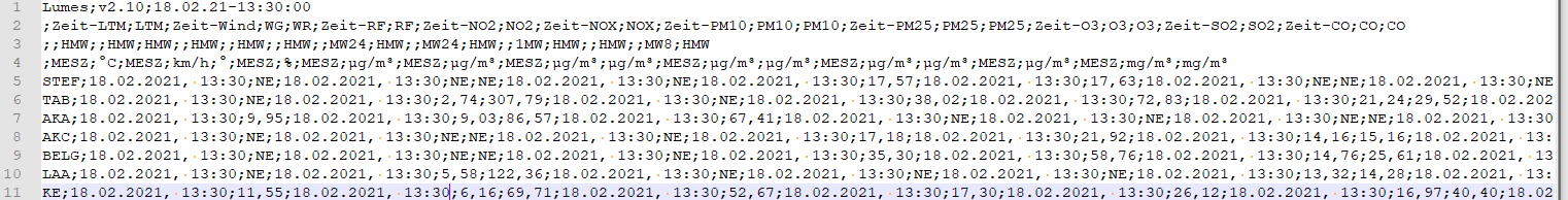
Let’s have a look at another real world example. Here, I am using the current air quality measurement for the city of Vienna as provided by data.gv.at. It can be downloaded from here. Again, here is a screen shot of the file:
Let’s go through the check list again:
What data do we expect? The meaning of each columns is explained on data.gv.at.
Air quality data (ozone (O3), nitrogen dioxide (NO2), nitrogen oxides (NOx), particulate matter (PM10 and PM2,5), sulfur dioxide (SO2), carbon monixide (CO)) from 17 stationary measuring points. The data originates from continuous measurements and is available in the form of half-hourly mean values which are updated every 30 minutes.
Which delimiter is used? The semicolon.
What is the line number of the first table row? The first data containing line is number 5.
Are there commments or a header? There are multiple headers, from line 2 to 4.
Is the number format “weird”? (E.g.
,instead of.for decimal seperator))? Yes,,instead of..Do rows contain text data? Some cells do, others contain times and dates.
The complex nature of this file means we are probably better off using pandas right away instead of trying our luck with numpy. Let’s give it a try:
lumes = pd.read_csv("data/lumesakt-v2.csv",
                    delimiter=";",
                    header=[1,2,3])
Unfortunately, this fails for some reason. Python tells us, that there is a UnicodeDecodeError. To understand that, we need to take a step back. Remember, when we talked about computers representing everything as ones and zeroes and the meaning of series of ones and zeros (or bytes) being just up to convention? The same is also true for (text) files. For text files, the convention used to interpret it’s contents are called “encoding” or “codec”. UTF-8 is one such codec and it is used as default in read_csv.
Unfortunately, even though the description of the file on data.gv.at claims the data is “utf8”, it is not. To find out which encoding was actually used, we can again use our editor. For example in Notepad++ the encoding is shown in the “Encoding” menu. Here, we see that “ANSI” encoding might have been used in this file. We can pass that as an optional argument.
lumes = pd.read_csv("data/lumesakt-v2.csv",
                    delimiter=";",
                    header=[1,2,3],
                   encoding="iso-8859-1")
lumes
| Unnamed: 0_level_0 | Zeit-LTM | LTM | Zeit-Wind | WG | WR | Zeit-RF | RF | Zeit-NO2 | NO2 | ... | PM25 | Zeit-O3 | O3 | Zeit-SO2 | SO2 | Zeit-CO | CO | ||||
|---|---|---|---|---|---|---|---|---|---|---|---|---|---|---|---|---|---|---|---|---|---|
| Unnamed: 0_level_1 | Unnamed: 1_level_1 | HMW | Unnamed: 3_level_1 | HMW | HMW | Unnamed: 6_level_1 | HMW | Unnamed: 8_level_1 | HMW | ... | MW24 | HMW | Unnamed: 18_level_1 | 1MW | HMW | Unnamed: 21_level_1 | HMW | Unnamed: 23_level_1 | MW8 | HMW | |
| Unnamed: 0_level_2 | MESZ | °C | MESZ | km/h | ° | MESZ | % | MESZ | µg/m³ | ... | µg/m³ | µg/m³ | MESZ | µg/m³ | µg/m³ | MESZ | µg/m³ | MESZ | mg/m³ | mg/m³ | |
| 0 | STEF | 18.02.2021, 13:30 | NE | 18.02.2021, 13:30 | NE | NE | 18.02.2021, 13:30 | NE | 18.02.2021, 13:30 | 17,57 | ... | NE | NE | 18.02.2021, 13:30 | 53,93 | 56,58 | 18.02.2021, 13:30 | 2,33 | 18.02.2021, 13:30 | NE | NE |
| 1 | TAB | 18.02.2021, 13:30 | NE | 18.02.2021, 13:30 | 2,74 | 307,79 | 18.02.2021, 13:30 | NE | 18.02.2021, 13:30 | 38,02 | ... | 9,09 | 10,45 | 18.02.2021, 13:30 | NE | NE | 18.02.2021, 13:30 | NE | 18.02.2021, 13:30 | 0,37 | 0,18 |
| 2 | AKA | 18.02.2021, 13:30 | 9,95 | 18.02.2021, 13:30 | 9,03 | 86,57 | 18.02.2021, 13:30 | 67,41 | 18.02.2021, 13:30 | NE | ... | NE | NE | 18.02.2021, 13:30 | NE | NE | 18.02.2021, 13:30 | NE | 18.02.2021, 13:30 | NE | NE |
| 3 | AKC | 18.02.2021, 13:30 | NE | 18.02.2021, 13:30 | NE | NE | 18.02.2021, 13:30 | NE | 18.02.2021, 13:30 | 17,18 | ... | 7,63 | 8,95 | 18.02.2021, 13:30 | NE | NE | 18.02.2021, 13:30 | NE | 18.02.2021, 13:30 | NE | NE |
| 4 | BELG | 18.02.2021, 13:30 | NE | 18.02.2021, 13:30 | NE | NE | 18.02.2021, 13:30 | NE | 18.02.2021, 13:30 | 35,30 | ... | 8,52 | 10,91 | 18.02.2021, 13:30 | NE | NE | 18.02.2021, 13:30 | NE | 18.02.2021, 13:30 | NE | NE |
| 5 | LAA | 18.02.2021, 13:30 | NE | 18.02.2021, 13:30 | 5,58 | 122,36 | 18.02.2021, 13:30 | NE | 18.02.2021, 13:30 | NE | ... | 7,88 | 7,90 | 18.02.2021, 13:30 | 18,19 | 18,77 | 18.02.2021, 13:30 | NE | 18.02.2021, 13:30 | NE | NE |
| 6 | KE | 18.02.2021, 13:30 | 11,55 | 18.02.2021, 13:30 | 6,16 | 69,71 | 18.02.2021, 13:30 | 52,67 | 18.02.2021, 13:30 | 17,30 | ... | 8,88 | 9,61 | 18.02.2021, 13:30 | NE | NE | 18.02.2021, 13:30 | 2,47 | 18.02.2021, 13:30 | NE | NE |
| 7 | A23 | 18.02.2021, 13:30 | 10,59 | 18.02.2021, 13:30 | 2,09 | 165,87 | 18.02.2021, 13:30 | 52,83 | 18.02.2021, 13:30 | 17,20 | ... | 8,06 | 6,96 | 18.02.2021, 13:30 | NE | NE | 18.02.2021, 13:30 | 4,85 | 18.02.2021, 13:30 | 0,36 | 0,19 |
| 8 | GAUD | 18.02.2021, 13:30 | 11,08 | 18.02.2021, 13:30 | NE | NE | 18.02.2021, 13:30 | 55,57 | 18.02.2021, 13:30 | 43,93 | ... | 7,90 | 11,09 | 18.02.2021, 13:30 | NE | NE | 18.02.2021, 13:30 | NE | 18.02.2021, 13:30 | NE | NE |
| 9 | MBA | 18.02.2021, 13:30 | NE | 18.02.2021, 13:30 | NE | NE | 18.02.2021, 13:30 | NE | 18.02.2021, 13:30 | 54,88 | ... | NE | NE | 18.02.2021, 13:30 | NE | NE | 18.02.2021, 13:30 | NE | 18.02.2021, 13:30 | 0,43 | 0,33 |
| 10 | KEND | 18.02.2021, 13:30 | NE | 18.02.2021, 13:30 | 6,73 | 94,39 | 18.02.2021, 13:30 | NE | 18.02.2021, 13:30 | 27,83 | ... | 6,88 | 10,64 | 18.02.2021, 13:30 | NE | NE | 18.02.2021, 13:30 | NE | 18.02.2021, 13:30 | NE | NE |
| 11 | SCHA | 18.02.2021, 13:30 | NE | 18.02.2021, 13:30 | 6,20 | 104,98 | 18.02.2021, 13:30 | NE | 18.02.2021, 13:00 | 15,02 | ... | 4,40 | 8,25 | 18.02.2021, 13:30 | NE | NE | 18.02.2021, 13:30 | 2,60 | 18.02.2021, 13:30 | NE | NE |
| 12 | JAEG | 18.02.2021, 13:30 | 10,49 | 18.02.2021, 13:30 | 10,81 | 130,05 | 18.02.2021, 13:30 | 55,03 | 18.02.2021, 13:30 | 10,58 | ... | NE | NE | 18.02.2021, 13:30 | 70,01 | 69,11 | 18.02.2021, 13:30 | NE | 18.02.2021, 13:30 | NE | NE |
| 13 | ZA | 18.02.2021, 13:30 | NE | 18.02.2021, 13:30 | NE | NE | 18.02.2021, 13:30 | NE | 18.02.2021, 13:30 | 12,52 | ... | NE | NE | 18.02.2021, 13:30 | 68,55 | 70,37 | 18.02.2021, 13:30 | 1,31 | 18.02.2021, 13:30 | NE | NE |
| 14 | FLO | 18.02.2021, 13:30 | NE | 18.02.2021, 13:30 | NE | NE | 18.02.2021, 13:30 | NE | 18.02.2021, 13:30 | 14,56 | ... | 5,85 | 6,52 | 18.02.2021, 13:30 | NE | NE | 18.02.2021, 13:30 | NE | 18.02.2021, 13:30 | NE | NE |
| 15 | LOB | 18.02.2021, 13:30 | 10,74 | 18.02.2021, 13:30 | 6,01 | 73,36 | 18.02.2021, 13:30 | 53,98 | 18.02.2021, 13:30 | 4,96 | ... | 5,17 | 4,45 | 18.02.2021, 13:30 | 70,32 | 74,10 | 18.02.2021, 13:30 | NE | 18.02.2021, 13:30 | NE | NE |
| 16 | STAD | 18.02.2021, 13:30 | NE | 18.02.2021, 13:30 | 6,37 | 13,98 | 18.02.2021, 13:30 | NE | 18.02.2021, 13:30 | 11,43 | ... | 7,74 | 7,81 | 18.02.2021, 13:30 | NE | NE | 18.02.2021, 13:30 | 1,97 | 18.02.2021, 13:30 | NE | NE |
| 17 | LIES | 18.02.2021, 13:30 | NE | 18.02.2021, 13:30 | 9,91 | 114,79 | 18.02.2021, 13:30 | NE | 18.02.2021, 13:30 | 25,04 | ... | 7,62 | 9,29 | 18.02.2021, 13:30 | NE | NE | 18.02.2021, 13:30 | NE | 18.02.2021, 13:30 | NE | NE |
| 18 | BC21 | 18.02.2021, 13:30 | 10,35 | 18.02.2021, 13:30 | 10,05 | 107,78 | 18.02.2021, 13:30 | 57,76 | 18.02.2021, 13:30 | NE | ... | NE | NE | 18.02.2021, 13:30 | NE | NE | 18.02.2021, 13:30 | NE | 18.02.2021, 13:30 | NE | NE |
19 rows × 26 columns
There are still some things that seem a bit fishy. First of all, there are quite a few instances of the string “NE” in the parsed table. “NE” probably stands for values that were either not available or not determined. We need to tell python to ignore these or rather set them to nan.
Second, there are also columns still containing the, as decimal separator. Since python always represents the decimal separator as . it seems these have not been parsed correctly. They are still represented as strings. To be sure, let’s check the type of one of these values:
lumes.loc[1, "WG"]
HMW  km/h    2,74
Name: 1, dtype: object
Unfortunately, that doesn’t look gread. The dtype of this value is stated to be “object”. A generic, catch all type that tells us, read_csv had no idea what to do with the data. Let’s check the other data types:
lumes.dtypes
Unnamed: 0_level_0  Unnamed: 0_level_1   Unnamed: 0_level_2    object
Zeit-LTM            Unnamed: 1_level_1   MESZ                  object
LTM                 HMW                  °C                    object
Zeit-Wind           Unnamed: 3_level_1   MESZ                  object
WG                  HMW                  km/h                  object
WR                  HMW                  °                     object
Zeit-RF             Unnamed: 6_level_1   MESZ                  object
RF                  HMW                  %                     object
Zeit-NO2            Unnamed: 8_level_1   MESZ                  object
NO2                 HMW                  µg/m³                 object
Zeit-NOX            Unnamed: 10_level_1  MESZ                  object
NOX                 HMW                  µg/m³                 object
Zeit-PM10           Unnamed: 12_level_1  MESZ                  object
PM10                MW24                 µg/m³                 object
                    HMW                  µg/m³                 object
Zeit-PM25           Unnamed: 15_level_1  MESZ                  object
PM25                MW24                 µg/m³                 object
                    HMW                  µg/m³                 object
Zeit-O3             Unnamed: 18_level_1  MESZ                  object
O3                  1MW                  µg/m³                 object
                    HMW                  µg/m³                 object
Zeit-SO2            Unnamed: 21_level_1  MESZ                  object
SO2                 HMW                  µg/m³                 object
Zeit-CO             Unnamed: 23_level_1  MESZ                  object
CO                  MW8                  mg/m³                 object
                    HMW                  mg/m³                 object
dtype: object
Again, dtype is object. So that didn’t work either.
We need to refine the arguments passed to read_csv a bit to actually get meaningful data here. Looking at the documentation of the function, we see several optional arguments that could be helpful.
na_values : scalar, str, list-like, or dict, optional
Additional strings to recognize as NA/NaN. If dict passed, specific per-column NA values. By default the following values are interpreted as NaN: ‘’, ‘#N/A’, ‘#N/A N/A’, ‘#NA’, ‘-1.#IND’, ‘-1.#QNAN’, ‘-NaN’, ‘-nan’, ‘1.#IND’, ‘1.#QNAN’, ‘
’, ‘N/A’, ‘NA’, ‘NULL’, ‘NaN’, ‘n/a’, ‘nan’, ‘null’.
decimal : str, default ‘.’
Character to recognize as decimal point (e.g. use ‘,’ for European data).
parse_dates : bool or list of int or names or list of lists or dict, default False The behavior is as follows:
boolean. If True -> try parsing the index.
list of int or names. e.g. If [1, 2, 3] -> try parsing columns 1, 2, 3 each as a separate date column.
list of lists. e.g. If [[1, 3]] -> combine columns 1 and 3 and parse as a single date column.
dict, e.g. {‘foo’ : [1, 3]} -> parse columns 1, 3 as date and call result ‘foo’
lumes = pd.read_csv("data/lumesakt-v2.csv",
                    delimiter=";",
                    na_values="NE",
                    decimal=",",
                    parse_dates=[1,3,6,8,10,12,15,18,21,23],
                    header=[1,2,3],
                    encoding="iso-8859-1")
lumes
| Unnamed: 0_level_0 | Zeit-LTM | LTM | Zeit-Wind | WG | WR | Zeit-RF | RF | Zeit-NO2 | NO2 | ... | PM25 | Zeit-O3 | O3 | Zeit-SO2 | SO2 | Zeit-CO | CO | ||||
|---|---|---|---|---|---|---|---|---|---|---|---|---|---|---|---|---|---|---|---|---|---|
| Unnamed: 0_level_1 | Unnamed: 1_level_1 | HMW | Unnamed: 3_level_1 | HMW | HMW | Unnamed: 6_level_1 | HMW | Unnamed: 8_level_1 | HMW | ... | MW24 | HMW | Unnamed: 18_level_1 | 1MW | HMW | Unnamed: 21_level_1 | HMW | Unnamed: 23_level_1 | MW8 | HMW | |
| Unnamed: 0_level_2 | MESZ | °C | MESZ | km/h | ° | MESZ | % | MESZ | µg/m³ | ... | µg/m³ | µg/m³ | MESZ | µg/m³ | µg/m³ | MESZ | µg/m³ | MESZ | mg/m³ | mg/m³ | |
| 0 | STEF | 2021-02-18 13:30:00 | NaN | 2021-02-18 13:30:00 | NaN | NaN | 2021-02-18 13:30:00 | NaN | 2021-02-18 13:30:00 | 17.57 | ... | NaN | NaN | 2021-02-18 13:30:00 | 53.93 | 56.58 | 2021-02-18 13:30:00 | 2.33 | 2021-02-18 13:30:00 | NaN | NaN |
| 1 | TAB | 2021-02-18 13:30:00 | NaN | 2021-02-18 13:30:00 | 2.74 | 307.79 | 2021-02-18 13:30:00 | NaN | 2021-02-18 13:30:00 | 38.02 | ... | 9.09 | 10.45 | 2021-02-18 13:30:00 | NaN | NaN | 2021-02-18 13:30:00 | NaN | 2021-02-18 13:30:00 | 0.37 | 0.18 |
| 2 | AKA | 2021-02-18 13:30:00 | 9.95 | 2021-02-18 13:30:00 | 9.03 | 86.57 | 2021-02-18 13:30:00 | 67.41 | 2021-02-18 13:30:00 | NaN | ... | NaN | NaN | 2021-02-18 13:30:00 | NaN | NaN | 2021-02-18 13:30:00 | NaN | 2021-02-18 13:30:00 | NaN | NaN |
| 3 | AKC | 2021-02-18 13:30:00 | NaN | 2021-02-18 13:30:00 | NaN | NaN | 2021-02-18 13:30:00 | NaN | 2021-02-18 13:30:00 | 17.18 | ... | 7.63 | 8.95 | 2021-02-18 13:30:00 | NaN | NaN | 2021-02-18 13:30:00 | NaN | 2021-02-18 13:30:00 | NaN | NaN |
| 4 | BELG | 2021-02-18 13:30:00 | NaN | 2021-02-18 13:30:00 | NaN | NaN | 2021-02-18 13:30:00 | NaN | 2021-02-18 13:30:00 | 35.30 | ... | 8.52 | 10.91 | 2021-02-18 13:30:00 | NaN | NaN | 2021-02-18 13:30:00 | NaN | 2021-02-18 13:30:00 | NaN | NaN |
| 5 | LAA | 2021-02-18 13:30:00 | NaN | 2021-02-18 13:30:00 | 5.58 | 122.36 | 2021-02-18 13:30:00 | NaN | 2021-02-18 13:30:00 | NaN | ... | 7.88 | 7.90 | 2021-02-18 13:30:00 | 18.19 | 18.77 | 2021-02-18 13:30:00 | NaN | 2021-02-18 13:30:00 | NaN | NaN |
| 6 | KE | 2021-02-18 13:30:00 | 11.55 | 2021-02-18 13:30:00 | 6.16 | 69.71 | 2021-02-18 13:30:00 | 52.67 | 2021-02-18 13:30:00 | 17.30 | ... | 8.88 | 9.61 | 2021-02-18 13:30:00 | NaN | NaN | 2021-02-18 13:30:00 | 2.47 | 2021-02-18 13:30:00 | NaN | NaN |
| 7 | A23 | 2021-02-18 13:30:00 | 10.59 | 2021-02-18 13:30:00 | 2.09 | 165.87 | 2021-02-18 13:30:00 | 52.83 | 2021-02-18 13:30:00 | 17.20 | ... | 8.06 | 6.96 | 2021-02-18 13:30:00 | NaN | NaN | 2021-02-18 13:30:00 | 4.85 | 2021-02-18 13:30:00 | 0.36 | 0.19 |
| 8 | GAUD | 2021-02-18 13:30:00 | 11.08 | 2021-02-18 13:30:00 | NaN | NaN | 2021-02-18 13:30:00 | 55.57 | 2021-02-18 13:30:00 | 43.93 | ... | 7.90 | 11.09 | 2021-02-18 13:30:00 | NaN | NaN | 2021-02-18 13:30:00 | NaN | 2021-02-18 13:30:00 | NaN | NaN |
| 9 | MBA | 2021-02-18 13:30:00 | NaN | 2021-02-18 13:30:00 | NaN | NaN | 2021-02-18 13:30:00 | NaN | 2021-02-18 13:30:00 | 54.88 | ... | NaN | NaN | 2021-02-18 13:30:00 | NaN | NaN | 2021-02-18 13:30:00 | NaN | 2021-02-18 13:30:00 | 0.43 | 0.33 |
| 10 | KEND | 2021-02-18 13:30:00 | NaN | 2021-02-18 13:30:00 | 6.73 | 94.39 | 2021-02-18 13:30:00 | NaN | 2021-02-18 13:30:00 | 27.83 | ... | 6.88 | 10.64 | 2021-02-18 13:30:00 | NaN | NaN | 2021-02-18 13:30:00 | NaN | 2021-02-18 13:30:00 | NaN | NaN |
| 11 | SCHA | 2021-02-18 13:30:00 | NaN | 2021-02-18 13:30:00 | 6.20 | 104.98 | 2021-02-18 13:30:00 | NaN | 2021-02-18 13:00:00 | 15.02 | ... | 4.40 | 8.25 | 2021-02-18 13:30:00 | NaN | NaN | 2021-02-18 13:30:00 | 2.60 | 2021-02-18 13:30:00 | NaN | NaN |
| 12 | JAEG | 2021-02-18 13:30:00 | 10.49 | 2021-02-18 13:30:00 | 10.81 | 130.05 | 2021-02-18 13:30:00 | 55.03 | 2021-02-18 13:30:00 | 10.58 | ... | NaN | NaN | 2021-02-18 13:30:00 | 70.01 | 69.11 | 2021-02-18 13:30:00 | NaN | 2021-02-18 13:30:00 | NaN | NaN |
| 13 | ZA | 2021-02-18 13:30:00 | NaN | 2021-02-18 13:30:00 | NaN | NaN | 2021-02-18 13:30:00 | NaN | 2021-02-18 13:30:00 | 12.52 | ... | NaN | NaN | 2021-02-18 13:30:00 | 68.55 | 70.37 | 2021-02-18 13:30:00 | 1.31 | 2021-02-18 13:30:00 | NaN | NaN |
| 14 | FLO | 2021-02-18 13:30:00 | NaN | 2021-02-18 13:30:00 | NaN | NaN | 2021-02-18 13:30:00 | NaN | 2021-02-18 13:30:00 | 14.56 | ... | 5.85 | 6.52 | 2021-02-18 13:30:00 | NaN | NaN | 2021-02-18 13:30:00 | NaN | 2021-02-18 13:30:00 | NaN | NaN |
| 15 | LOB | 2021-02-18 13:30:00 | 10.74 | 2021-02-18 13:30:00 | 6.01 | 73.36 | 2021-02-18 13:30:00 | 53.98 | 2021-02-18 13:30:00 | 4.96 | ... | 5.17 | 4.45 | 2021-02-18 13:30:00 | 70.32 | 74.10 | 2021-02-18 13:30:00 | NaN | 2021-02-18 13:30:00 | NaN | NaN |
| 16 | STAD | 2021-02-18 13:30:00 | NaN | 2021-02-18 13:30:00 | 6.37 | 13.98 | 2021-02-18 13:30:00 | NaN | 2021-02-18 13:30:00 | 11.43 | ... | 7.74 | 7.81 | 2021-02-18 13:30:00 | NaN | NaN | 2021-02-18 13:30:00 | 1.97 | 2021-02-18 13:30:00 | NaN | NaN |
| 17 | LIES | 2021-02-18 13:30:00 | NaN | 2021-02-18 13:30:00 | 9.91 | 114.79 | 2021-02-18 13:30:00 | NaN | 2021-02-18 13:30:00 | 25.04 | ... | 7.62 | 9.29 | 2021-02-18 13:30:00 | NaN | NaN | 2021-02-18 13:30:00 | NaN | 2021-02-18 13:30:00 | NaN | NaN |
| 18 | BC21 | 2021-02-18 13:30:00 | 10.35 | 2021-02-18 13:30:00 | 10.05 | 107.78 | 2021-02-18 13:30:00 | 57.76 | 2021-02-18 13:30:00 | NaN | ... | NaN | NaN | 2021-02-18 13:30:00 | NaN | NaN | 2021-02-18 13:30:00 | NaN | 2021-02-18 13:30:00 | NaN | NaN |
19 rows × 26 columns
Let’s check again if all columns are now recognized correctly:
lumes.dtypes
Unnamed: 0_level_0  Unnamed: 0_level_1   Unnamed: 0_level_2            object
Zeit-LTM            Unnamed: 1_level_1   MESZ                  datetime64[ns]
LTM                 HMW                  °C                           float64
Zeit-Wind           Unnamed: 3_level_1   MESZ                  datetime64[ns]
WG                  HMW                  km/h                         float64
WR                  HMW                  °                            float64
Zeit-RF             Unnamed: 6_level_1   MESZ                  datetime64[ns]
RF                  HMW                  %                            float64
Zeit-NO2            Unnamed: 8_level_1   MESZ                  datetime64[ns]
NO2                 HMW                  µg/m³                        float64
Zeit-NOX            Unnamed: 10_level_1  MESZ                  datetime64[ns]
NOX                 HMW                  µg/m³                        float64
Zeit-PM10           Unnamed: 12_level_1  MESZ                  datetime64[ns]
PM10                MW24                 µg/m³                        float64
                    HMW                  µg/m³                        float64
Zeit-PM25           Unnamed: 15_level_1  MESZ                  datetime64[ns]
PM25                MW24                 µg/m³                        float64
                    HMW                  µg/m³                        float64
Zeit-O3             Unnamed: 18_level_1  MESZ                  datetime64[ns]
O3                  1MW                  µg/m³                        float64
                    HMW                  µg/m³                        float64
Zeit-SO2            Unnamed: 21_level_1  MESZ                  datetime64[ns]
SO2                 HMW                  µg/m³                        float64
Zeit-CO             Unnamed: 23_level_1  MESZ                  datetime64[ns]
CO                  MW8                  mg/m³                        float64
                    HMW                  mg/m³                        float64
dtype: object
Everything that has “Zeit” (for “time”) in its name is a datetime64, everything else is float64. Except for “Unnamed”, which contains strings encoding the location of each measurement point. Let’s rename it.
lumes = lumes.rename(columns={"Unnamed: 0_level_0":"Standort"})
lumes
| Standort | Zeit-LTM | LTM | Zeit-Wind | WG | WR | Zeit-RF | RF | Zeit-NO2 | NO2 | ... | PM25 | Zeit-O3 | O3 | Zeit-SO2 | SO2 | Zeit-CO | CO | ||||
|---|---|---|---|---|---|---|---|---|---|---|---|---|---|---|---|---|---|---|---|---|---|
| Unnamed: 0_level_1 | Unnamed: 1_level_1 | HMW | Unnamed: 3_level_1 | HMW | HMW | Unnamed: 6_level_1 | HMW | Unnamed: 8_level_1 | HMW | ... | MW24 | HMW | Unnamed: 18_level_1 | 1MW | HMW | Unnamed: 21_level_1 | HMW | Unnamed: 23_level_1 | MW8 | HMW | |
| Unnamed: 0_level_2 | MESZ | °C | MESZ | km/h | ° | MESZ | % | MESZ | µg/m³ | ... | µg/m³ | µg/m³ | MESZ | µg/m³ | µg/m³ | MESZ | µg/m³ | MESZ | mg/m³ | mg/m³ | |
| 0 | STEF | 2021-02-18 13:30:00 | NaN | 2021-02-18 13:30:00 | NaN | NaN | 2021-02-18 13:30:00 | NaN | 2021-02-18 13:30:00 | 17.57 | ... | NaN | NaN | 2021-02-18 13:30:00 | 53.93 | 56.58 | 2021-02-18 13:30:00 | 2.33 | 2021-02-18 13:30:00 | NaN | NaN |
| 1 | TAB | 2021-02-18 13:30:00 | NaN | 2021-02-18 13:30:00 | 2.74 | 307.79 | 2021-02-18 13:30:00 | NaN | 2021-02-18 13:30:00 | 38.02 | ... | 9.09 | 10.45 | 2021-02-18 13:30:00 | NaN | NaN | 2021-02-18 13:30:00 | NaN | 2021-02-18 13:30:00 | 0.37 | 0.18 |
| 2 | AKA | 2021-02-18 13:30:00 | 9.95 | 2021-02-18 13:30:00 | 9.03 | 86.57 | 2021-02-18 13:30:00 | 67.41 | 2021-02-18 13:30:00 | NaN | ... | NaN | NaN | 2021-02-18 13:30:00 | NaN | NaN | 2021-02-18 13:30:00 | NaN | 2021-02-18 13:30:00 | NaN | NaN |
| 3 | AKC | 2021-02-18 13:30:00 | NaN | 2021-02-18 13:30:00 | NaN | NaN | 2021-02-18 13:30:00 | NaN | 2021-02-18 13:30:00 | 17.18 | ... | 7.63 | 8.95 | 2021-02-18 13:30:00 | NaN | NaN | 2021-02-18 13:30:00 | NaN | 2021-02-18 13:30:00 | NaN | NaN |
| 4 | BELG | 2021-02-18 13:30:00 | NaN | 2021-02-18 13:30:00 | NaN | NaN | 2021-02-18 13:30:00 | NaN | 2021-02-18 13:30:00 | 35.30 | ... | 8.52 | 10.91 | 2021-02-18 13:30:00 | NaN | NaN | 2021-02-18 13:30:00 | NaN | 2021-02-18 13:30:00 | NaN | NaN |
| 5 | LAA | 2021-02-18 13:30:00 | NaN | 2021-02-18 13:30:00 | 5.58 | 122.36 | 2021-02-18 13:30:00 | NaN | 2021-02-18 13:30:00 | NaN | ... | 7.88 | 7.90 | 2021-02-18 13:30:00 | 18.19 | 18.77 | 2021-02-18 13:30:00 | NaN | 2021-02-18 13:30:00 | NaN | NaN |
| 6 | KE | 2021-02-18 13:30:00 | 11.55 | 2021-02-18 13:30:00 | 6.16 | 69.71 | 2021-02-18 13:30:00 | 52.67 | 2021-02-18 13:30:00 | 17.30 | ... | 8.88 | 9.61 | 2021-02-18 13:30:00 | NaN | NaN | 2021-02-18 13:30:00 | 2.47 | 2021-02-18 13:30:00 | NaN | NaN |
| 7 | A23 | 2021-02-18 13:30:00 | 10.59 | 2021-02-18 13:30:00 | 2.09 | 165.87 | 2021-02-18 13:30:00 | 52.83 | 2021-02-18 13:30:00 | 17.20 | ... | 8.06 | 6.96 | 2021-02-18 13:30:00 | NaN | NaN | 2021-02-18 13:30:00 | 4.85 | 2021-02-18 13:30:00 | 0.36 | 0.19 |
| 8 | GAUD | 2021-02-18 13:30:00 | 11.08 | 2021-02-18 13:30:00 | NaN | NaN | 2021-02-18 13:30:00 | 55.57 | 2021-02-18 13:30:00 | 43.93 | ... | 7.90 | 11.09 | 2021-02-18 13:30:00 | NaN | NaN | 2021-02-18 13:30:00 | NaN | 2021-02-18 13:30:00 | NaN | NaN |
| 9 | MBA | 2021-02-18 13:30:00 | NaN | 2021-02-18 13:30:00 | NaN | NaN | 2021-02-18 13:30:00 | NaN | 2021-02-18 13:30:00 | 54.88 | ... | NaN | NaN | 2021-02-18 13:30:00 | NaN | NaN | 2021-02-18 13:30:00 | NaN | 2021-02-18 13:30:00 | 0.43 | 0.33 |
| 10 | KEND | 2021-02-18 13:30:00 | NaN | 2021-02-18 13:30:00 | 6.73 | 94.39 | 2021-02-18 13:30:00 | NaN | 2021-02-18 13:30:00 | 27.83 | ... | 6.88 | 10.64 | 2021-02-18 13:30:00 | NaN | NaN | 2021-02-18 13:30:00 | NaN | 2021-02-18 13:30:00 | NaN | NaN |
| 11 | SCHA | 2021-02-18 13:30:00 | NaN | 2021-02-18 13:30:00 | 6.20 | 104.98 | 2021-02-18 13:30:00 | NaN | 2021-02-18 13:00:00 | 15.02 | ... | 4.40 | 8.25 | 2021-02-18 13:30:00 | NaN | NaN | 2021-02-18 13:30:00 | 2.60 | 2021-02-18 13:30:00 | NaN | NaN |
| 12 | JAEG | 2021-02-18 13:30:00 | 10.49 | 2021-02-18 13:30:00 | 10.81 | 130.05 | 2021-02-18 13:30:00 | 55.03 | 2021-02-18 13:30:00 | 10.58 | ... | NaN | NaN | 2021-02-18 13:30:00 | 70.01 | 69.11 | 2021-02-18 13:30:00 | NaN | 2021-02-18 13:30:00 | NaN | NaN |
| 13 | ZA | 2021-02-18 13:30:00 | NaN | 2021-02-18 13:30:00 | NaN | NaN | 2021-02-18 13:30:00 | NaN | 2021-02-18 13:30:00 | 12.52 | ... | NaN | NaN | 2021-02-18 13:30:00 | 68.55 | 70.37 | 2021-02-18 13:30:00 | 1.31 | 2021-02-18 13:30:00 | NaN | NaN |
| 14 | FLO | 2021-02-18 13:30:00 | NaN | 2021-02-18 13:30:00 | NaN | NaN | 2021-02-18 13:30:00 | NaN | 2021-02-18 13:30:00 | 14.56 | ... | 5.85 | 6.52 | 2021-02-18 13:30:00 | NaN | NaN | 2021-02-18 13:30:00 | NaN | 2021-02-18 13:30:00 | NaN | NaN |
| 15 | LOB | 2021-02-18 13:30:00 | 10.74 | 2021-02-18 13:30:00 | 6.01 | 73.36 | 2021-02-18 13:30:00 | 53.98 | 2021-02-18 13:30:00 | 4.96 | ... | 5.17 | 4.45 | 2021-02-18 13:30:00 | 70.32 | 74.10 | 2021-02-18 13:30:00 | NaN | 2021-02-18 13:30:00 | NaN | NaN |
| 16 | STAD | 2021-02-18 13:30:00 | NaN | 2021-02-18 13:30:00 | 6.37 | 13.98 | 2021-02-18 13:30:00 | NaN | 2021-02-18 13:30:00 | 11.43 | ... | 7.74 | 7.81 | 2021-02-18 13:30:00 | NaN | NaN | 2021-02-18 13:30:00 | 1.97 | 2021-02-18 13:30:00 | NaN | NaN |
| 17 | LIES | 2021-02-18 13:30:00 | NaN | 2021-02-18 13:30:00 | 9.91 | 114.79 | 2021-02-18 13:30:00 | NaN | 2021-02-18 13:30:00 | 25.04 | ... | 7.62 | 9.29 | 2021-02-18 13:30:00 | NaN | NaN | 2021-02-18 13:30:00 | NaN | 2021-02-18 13:30:00 | NaN | NaN |
| 18 | BC21 | 2021-02-18 13:30:00 | 10.35 | 2021-02-18 13:30:00 | 10.05 | 107.78 | 2021-02-18 13:30:00 | 57.76 | 2021-02-18 13:30:00 | NaN | ... | NaN | NaN | 2021-02-18 13:30:00 | NaN | NaN | 2021-02-18 13:30:00 | NaN | 2021-02-18 13:30:00 | NaN | NaN |
19 rows × 26 columns
We can now use this dataframe to check where the highest value of a parameter, e.g. the PM25 particle count, was recorded.
lumes.Standort.iloc[lumes.PM25.HMW.idxmax()]
| Unnamed: 0_level_1 | |
|---|---|
| Unnamed: 0_level_2 | |
| 8 | GAUD |
GAUD is the abreviation of a station in Gaudzendorf, right next to the Gürtel.
7.2. MS Excel and LibreOffice Calc
One option to load data from an Excel / LO Calc file is to export it as CSV, of course. However, pandas also has the capability to directly import from the native formats of these programs. The function to use is pandas.read_excel.
The example we are going to look at now consists of multi sheet excel file that is used to keep track of a process parameters in a mineral water plant. The upper an lower limits of ion concentration is given by Austrian law - minimum levels are required to still call the product “Mineralwasser”, maximum levels have to be kept for safety and public health reasons. (The data set is entirely artificial).
For each quarter, once a week a sample is take and analyzed via ion chromatography. The values are then copied by a lab technician into an Excel sheet and checked by the manager of the plant lab. Results are compiled by quarter and archived. The sheet for a quarter looks like this:
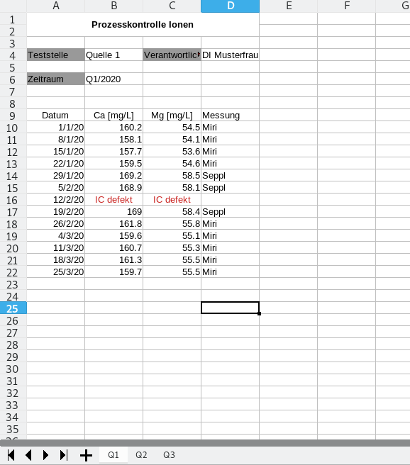
We have four columns containing data, and some additional meta data. Let’s have a look at the documentation of the pd.read_excel function to figure out how to call it:
help(pd.read_excel)
Help on function read_excel in module pandas.io.excel._base:

read_excel(io, sheet_name=0, header=0, names=None, index_col=None, usecols=None, squeeze=False, dtype=None, engine=None, converters=None, true_values=None, false_values=None, skiprows=None, nrows=None, na_values=None, keep_default_na=True, na_filter=True, verbose=False, parse_dates=False, date_parser=None, thousands=None, comment=None, skipfooter=0, convert_float=True, mangle_dupe_cols=True, storage_options: Optional[Dict[str, Any]] = None)
    Read an Excel file into a pandas DataFrame.

    Supports `xls`, `xlsx`, `xlsm`, `xlsb`, `odf`, `ods` and `odt` file extensions
    read from a local filesystem or URL. Supports an option to read
    a single sheet or a list of sheets.

    Parameters
    ----------
    io : str, bytes, ExcelFile, xlrd.Book, path object, or file-like object
        Any valid string path is acceptable. The string could be a URL. Valid
        URL schemes include http, ftp, s3, and file. For file URLs, a host is
        expected. A local file could be: ``file://localhost/path/to/table.xlsx``.

        If you want to pass in a path object, pandas accepts any ``os.PathLike``.

        By file-like object, we refer to objects with a ``read()`` method,
        such as a file handle (e.g. via builtin ``open`` function)
        or ``StringIO``.
    sheet_name : str, int, list, or None, default 0
        Strings are used for sheet names. Integers are used in zero-indexed
        sheet positions. Lists of strings/integers are used to request
        multiple sheets. Specify None to get all sheets.

        Available cases:

        * Defaults to ``0``: 1st sheet as a `DataFrame`
        * ``1``: 2nd sheet as a `DataFrame`
        * ``"Sheet1"``: Load sheet with name "Sheet1"
        * ``[0, 1, "Sheet5"]``: Load first, second and sheet named "Sheet5"
          as a dict of `DataFrame`
        * None: All sheets.

    header : int, list of int, default 0
        Row (0-indexed) to use for the column labels of the parsed
        DataFrame. If a list of integers is passed those row positions will
        be combined into a ``MultiIndex``. Use None if there is no header.
    names : array-like, default None
        List of column names to use. If file contains no header row,
        then you should explicitly pass header=None.
    index_col : int, list of int, default None
        Column (0-indexed) to use as the row labels of the DataFrame.
        Pass None if there is no such column.  If a list is passed,
        those columns will be combined into a ``MultiIndex``.  If a
        subset of data is selected with ``usecols``, index_col
        is based on the subset.
    usecols : int, str, list-like, or callable default None
        * If None, then parse all columns.
        * If str, then indicates comma separated list of Excel column letters
          and column ranges (e.g. "A:E" or "A,C,E:F"). Ranges are inclusive of
          both sides.
        * If list of int, then indicates list of column numbers to be parsed.
        * If list of string, then indicates list of column names to be parsed.

          .. versionadded:: 0.24.0

        * If callable, then evaluate each column name against it and parse the
          column if the callable returns ``True``.

        Returns a subset of the columns according to behavior above.

          .. versionadded:: 0.24.0

    squeeze : bool, default False
        If the parsed data only contains one column then return a Series.
    dtype : Type name or dict of column -> type, default None
        Data type for data or columns. E.g. {'a': np.float64, 'b': np.int32}
        Use `object` to preserve data as stored in Excel and not interpret dtype.
        If converters are specified, they will be applied INSTEAD
        of dtype conversion.
    engine : str, default None
        If io is not a buffer or path, this must be set to identify io.
        Supported engines: "xlrd", "openpyxl", "odf", "pyxlsb".
        Engine compatibility :

        - "xlrd" supports old-style Excel files (.xls).
        - "openpyxl" supports newer Excel file formats.
        - "odf" supports OpenDocument file formats (.odf, .ods, .odt).
        - "pyxlsb" supports Binary Excel files.

        .. versionchanged:: 1.2.0
            The engine `xlrd <https://xlrd.readthedocs.io/en/latest/>`_
            now only supports old-style ``.xls`` files.
            When ``engine=None``, the following logic will be
            used to determine the engine:

           - If ``path_or_buffer`` is an OpenDocument format (.odf, .ods, .odt),
             then `odf <https://pypi.org/project/odfpy/>`_ will be used.
           - Otherwise if ``path_or_buffer`` is an xls format,
             ``xlrd`` will be used.
           - Otherwise if `openpyxl <https://pypi.org/project/openpyxl/>`_ is installed,
             then ``openpyxl`` will be used.
           - Otherwise if ``xlrd >= 2.0`` is installed, a ``ValueError`` will be raised.
           - Otherwise ``xlrd`` will be used and a ``FutureWarning`` will be raised. This
             case will raise a ``ValueError`` in a future version of pandas.

    converters : dict, default None
        Dict of functions for converting values in certain columns. Keys can
        either be integers or column labels, values are functions that take one
        input argument, the Excel cell content, and return the transformed
        content.
    true_values : list, default None
        Values to consider as True.
    false_values : list, default None
        Values to consider as False.
    skiprows : list-like, int, or callable, optional
        Line numbers to skip (0-indexed) or number of lines to skip (int) at the
        start of the file. If callable, the callable function will be evaluated
        against the row indices, returning True if the row should be skipped and
        False otherwise. An example of a valid callable argument would be ``lambda
        x: x in [0, 2]``.
    nrows : int, default None
        Number of rows to parse.
    na_values : scalar, str, list-like, or dict, default None
        Additional strings to recognize as NA/NaN. If dict passed, specific
        per-column NA values. By default the following values are interpreted
        as NaN: '', '#N/A', '#N/A N/A', '#NA', '-1.#IND', '-1.#QNAN', '-NaN', '-nan',
        '1.#IND', '1.#QNAN', '<NA>', 'N/A', 'NA', 'NULL', 'NaN', 'n/a',
        'nan', 'null'.
    keep_default_na : bool, default True
        Whether or not to include the default NaN values when parsing the data.
        Depending on whether `na_values` is passed in, the behavior is as follows:

        * If `keep_default_na` is True, and `na_values` are specified, `na_values`
          is appended to the default NaN values used for parsing.
        * If `keep_default_na` is True, and `na_values` are not specified, only
          the default NaN values are used for parsing.
        * If `keep_default_na` is False, and `na_values` are specified, only
          the NaN values specified `na_values` are used for parsing.
        * If `keep_default_na` is False, and `na_values` are not specified, no
          strings will be parsed as NaN.

        Note that if `na_filter` is passed in as False, the `keep_default_na` and
        `na_values` parameters will be ignored.
    na_filter : bool, default True
        Detect missing value markers (empty strings and the value of na_values). In
        data without any NAs, passing na_filter=False can improve the performance
        of reading a large file.
    verbose : bool, default False
        Indicate number of NA values placed in non-numeric columns.
    parse_dates : bool, list-like, or dict, default False
        The behavior is as follows:

        * bool. If True -> try parsing the index.
        * list of int or names. e.g. If [1, 2, 3] -> try parsing columns 1, 2, 3
          each as a separate date column.
        * list of lists. e.g.  If [[1, 3]] -> combine columns 1 and 3 and parse as
          a single date column.
        * dict, e.g. {'foo' : [1, 3]} -> parse columns 1, 3 as date and call
          result 'foo'

        If a column or index contains an unparseable date, the entire column or
        index will be returned unaltered as an object data type. If you don`t want to
        parse some cells as date just change their type in Excel to "Text".
        For non-standard datetime parsing, use ``pd.to_datetime`` after ``pd.read_excel``.

        Note: A fast-path exists for iso8601-formatted dates.
    date_parser : function, optional
        Function to use for converting a sequence of string columns to an array of
        datetime instances. The default uses ``dateutil.parser.parser`` to do the
        conversion. Pandas will try to call `date_parser` in three different ways,
        advancing to the next if an exception occurs: 1) Pass one or more arrays
        (as defined by `parse_dates`) as arguments; 2) concatenate (row-wise) the
        string values from the columns defined by `parse_dates` into a single array
        and pass that; and 3) call `date_parser` once for each row using one or
        more strings (corresponding to the columns defined by `parse_dates`) as
        arguments.
    thousands : str, default None
        Thousands separator for parsing string columns to numeric.  Note that
        this parameter is only necessary for columns stored as TEXT in Excel,
        any numeric columns will automatically be parsed, regardless of display
        format.
    comment : str, default None
        Comments out remainder of line. Pass a character or characters to this
        argument to indicate comments in the input file. Any data between the
        comment string and the end of the current line is ignored.
    skipfooter : int, default 0
        Rows at the end to skip (0-indexed).
    convert_float : bool, default True
        Convert integral floats to int (i.e., 1.0 --> 1). If False, all numeric
        data will be read in as floats: Excel stores all numbers as floats
        internally.
    mangle_dupe_cols : bool, default True
        Duplicate columns will be specified as 'X', 'X.1', ...'X.N', rather than
        'X'...'X'. Passing in False will cause data to be overwritten if there
        are duplicate names in the columns.
    storage_options : dict, optional
        Extra options that make sense for a particular storage connection, e.g.
        host, port, username, password, etc., if using a URL that will
        be parsed by ``fsspec``, e.g., starting "s3://", "gcs://". An error
        will be raised if providing this argument with a local path or
        a file-like buffer. See the fsspec and backend storage implementation
        docs for the set of allowed keys and values.

        .. versionadded:: 1.2.0

    Returns
    -------
    DataFrame or dict of DataFrames
        DataFrame from the passed in Excel file. See notes in sheet_name
        argument for more information on when a dict of DataFrames is returned.

    See Also
    --------
    DataFrame.to_excel : Write DataFrame to an Excel file.
    DataFrame.to_csv : Write DataFrame to a comma-separated values (csv) file.
    read_csv : Read a comma-separated values (csv) file into DataFrame.
    read_fwf : Read a table of fixed-width formatted lines into DataFrame.

    Examples
    --------
    The file can be read using the file name as string or an open file object:

    >>> pd.read_excel('tmp.xlsx', index_col=0)  # doctest: +SKIP
           Name  Value
    0   string1      1
    1   string2      2
    2  #Comment      3

    >>> pd.read_excel(open('tmp.xlsx', 'rb'),
    ...               sheet_name='Sheet3')  # doctest: +SKIP
       Unnamed: 0      Name  Value
    0           0   string1      1
    1           1   string2      2
    2           2  #Comment      3

    Index and header can be specified via the `index_col` and `header` arguments

    >>> pd.read_excel('tmp.xlsx', index_col=None, header=None)  # doctest: +SKIP
         0         1      2
    0  NaN      Name  Value
    1  0.0   string1      1
    2  1.0   string2      2
    3  2.0  #Comment      3

    Column types are inferred but can be explicitly specified

    >>> pd.read_excel('tmp.xlsx', index_col=0,
    ...               dtype={'Name': str, 'Value': float})  # doctest: +SKIP
           Name  Value
    0   string1    1.0
    1   string2    2.0
    2  #Comment    3.0

    True, False, and NA values, and thousands separators have defaults,
    but can be explicitly specified, too. Supply the values you would like
    as strings or lists of strings!

    >>> pd.read_excel('tmp.xlsx', index_col=0,
    ...               na_values=['string1', 'string2'])  # doctest: +SKIP
           Name  Value
    0       NaN      1
    1       NaN      2
    2  #Comment      3

    Comment lines in the excel input file can be skipped using the `comment` kwarg

    >>> pd.read_excel('tmp.xlsx', index_col=0, comment='#')  # doctest: +SKIP
          Name  Value
    0  string1    1.0
    1  string2    2.0
    2     None    NaN
io is the path to our file.The first row of our data set (the header) is in line 9 (therefore skiprows is 8).
xlsxsheet = pd.read_excel("data/mineralwasser.xls",
              skiprows=8)
xlsxsheet
| Datum | Ca [mg/L] | Mg [mg/L] | Messung | |
|---|---|---|---|---|
| 0 | 2020-01-01 | 160.2 | 54.5 | Miri |
| 1 | 2020-01-08 | 158.1 | 54.1 | Miri |
| 2 | 2020-01-15 | 157.7 | 53.6 | Miri |
| 3 | 2020-01-22 | 159.5 | 54.6 | Miri |
| 4 | 2020-01-29 | 169.2 | 58.5 | Seppl |
| 5 | 2020-02-05 | 168.9 | 58.1 | Seppl |
| 6 | 2020-02-12 | IC defekt | IC defekt | NaN |
| 7 | 2020-02-19 | 169 | 58.4 | Seppl |
| 8 | 2020-02-26 | 161.8 | 55.8 | Miri |
| 9 | 2020-03-04 | 159.6 | 55.1 | Miri |
| 10 | 2020-03-11 | 160.7 | 55.3 | Miri |
| 11 | 2020-03-18 | 161.3 | 55.5 | Miri |
| 12 | 2020-03-25 | 159.7 | 55.5 | Miri |
This looks nice, but we run into a similar problem as with CSV files:
There is one day here, where the IC was broken. Since all data types in a column need to be the same, pandas defaults to the least common denominator between strings and floats, the generic “object”. We will add the string “IC defekt” to the list of na_values to make sure pandas transcribes these columns correctly.
xlsxsheet["Ca [mg/L]"]
0         160.2
1         158.1
2         157.7
3         159.5
4         169.2
5         168.9
6     IC defekt
7           169
8         161.8
9         159.6
10        160.7
11        161.3
12        159.7
Name: Ca [mg/L], dtype: object
xlsxsheet = pd.read_excel("data/mineralwasser.xls",
              skiprows=8,
            na_values="IC defekt"
                         )
xlsxsheet
| Datum | Ca [mg/L] | Mg [mg/L] | Messung | |
|---|---|---|---|---|
| 0 | 2020-01-01 | 160.2 | 54.5 | Miri |
| 1 | 2020-01-08 | 158.1 | 54.1 | Miri |
| 2 | 2020-01-15 | 157.7 | 53.6 | Miri |
| 3 | 2020-01-22 | 159.5 | 54.6 | Miri |
| 4 | 2020-01-29 | 169.2 | 58.5 | Seppl |
| 5 | 2020-02-05 | 168.9 | 58.1 | Seppl |
| 6 | 2020-02-12 | NaN | NaN | NaN |
| 7 | 2020-02-19 | 169.0 | 58.4 | Seppl |
| 8 | 2020-02-26 | 161.8 | 55.8 | Miri |
| 9 | 2020-03-04 | 159.6 | 55.1 | Miri |
| 10 | 2020-03-11 | 160.7 | 55.3 | Miri |
| 11 | 2020-03-18 | 161.3 | 55.5 | Miri |
| 12 | 2020-03-25 | 159.7 | 55.5 | Miri |
Now, we only have one sheet loaded, but there are three sheets in our data set. Pandas has the optional argument sheet_name that accepts a list of sheet names. We can also pass None there to get all sheets.
xlsxsheets = pd.read_excel("data/mineralwasser.xls",
              skiprows=8,
              na_values="IC defekt",
              sheet_name=None)
xlsxsheets
{'Q1':         Datum  Ca [mg/L]  Mg [mg/L] Messung
 0  2020-01-01      160.2       54.5    Miri
 1  2020-01-08      158.1       54.1    Miri
 2  2020-01-15      157.7       53.6    Miri
 3  2020-01-22      159.5       54.6    Miri
 4  2020-01-29      169.2       58.5   Seppl
 5  2020-02-05      168.9       58.1   Seppl
 6  2020-02-12        NaN        NaN     NaN
 7  2020-02-19      169.0       58.4   Seppl
 8  2020-02-26      161.8       55.8    Miri
 9  2020-03-04      159.6       55.1    Miri
 10 2020-03-11      160.7       55.3    Miri
 11 2020-03-18      161.3       55.5    Miri
 12 2020-03-25      159.7       55.5    Miri,
 'Q2':         Datum  Ca [mg/L]  Mg [mg/L] Messung
 0  2020-04-01      154.9       53.3   Seppl
 1  2020-04-08      161.1       54.8   Seppl
 2  2020-04-15      158.7       55.0    Miri
 3  2020-04-22      159.6       55.2    Miri
 4  2020-04-29      159.3       54.8    Miri
 5  2020-05-06      159.6       55.1    Miri
 6  2020-05-13      160.3       55.1    Miri
 7  2020-05-20      157.3       54.4   Seppl
 8  2020-05-27      164.3       56.4   Seppl
 9  2020-06-03      166.8       57.0   Seppl
 10 2020-06-10      149.4       51.1   Seppl
 11 2020-06-17      167.9       58.1   Seppl
 12 2020-06-24      172.8       59.1   Seppl,
 'Q3':         Datum  Ca [mg/L]  Mg [mg/L] Messung
 0  2020-07-01      154.8       53.5   Seppl
 1  2020-07-08      160.8       55.3   Seppl
 2  2020-07-15      166.5       57.6   Seppl
 3  2020-07-22      158.1       54.6   Seppl
 4  2020-07-29      152.1       52.5   Seppl
 5  2020-08-05      161.3       55.8   Seppl
 6  2020-08-12      158.1       54.5   Seppl
 7  2020-08-19      159.7       54.9   Seppl
 8  2020-08-26      154.8       53.5   Seppl
 9  2020-09-02      155.7       53.8   Seppl
 10 2020-09-09      150.7       52.1   Seppl
 11 2020-09-16      151.0       52.0    Miri
 12 2020-09-23      148.7       51.2    Miri}
This results in a dictionary containing DataFrames (because pandas can’t rely on the fact that all sheets in an Excel file will have the same columns). We have to merge them manually. Doing so for the dictionary uses the dictionary keys (the sheet names) as part of a two level index:
ion_dataset = pd.concat(xlsxsheets, axis=0)
ion_dataset
| Datum | Ca [mg/L] | Mg [mg/L] | Messung | ||
|---|---|---|---|---|---|
| Q1 | 0 | 2020-01-01 | 160.2 | 54.5 | Miri |
| 1 | 2020-01-08 | 158.1 | 54.1 | Miri | |
| 2 | 2020-01-15 | 157.7 | 53.6 | Miri | |
| 3 | 2020-01-22 | 159.5 | 54.6 | Miri | |
| 4 | 2020-01-29 | 169.2 | 58.5 | Seppl | |
| 5 | 2020-02-05 | 168.9 | 58.1 | Seppl | |
| 6 | 2020-02-12 | NaN | NaN | NaN | |
| 7 | 2020-02-19 | 169.0 | 58.4 | Seppl | |
| 8 | 2020-02-26 | 161.8 | 55.8 | Miri | |
| 9 | 2020-03-04 | 159.6 | 55.1 | Miri | |
| 10 | 2020-03-11 | 160.7 | 55.3 | Miri | |
| 11 | 2020-03-18 | 161.3 | 55.5 | Miri | |
| 12 | 2020-03-25 | 159.7 | 55.5 | Miri | |
| Q2 | 0 | 2020-04-01 | 154.9 | 53.3 | Seppl |
| 1 | 2020-04-08 | 161.1 | 54.8 | Seppl | |
| 2 | 2020-04-15 | 158.7 | 55.0 | Miri | |
| 3 | 2020-04-22 | 159.6 | 55.2 | Miri | |
| 4 | 2020-04-29 | 159.3 | 54.8 | Miri | |
| 5 | 2020-05-06 | 159.6 | 55.1 | Miri | |
| 6 | 2020-05-13 | 160.3 | 55.1 | Miri | |
| 7 | 2020-05-20 | 157.3 | 54.4 | Seppl | |
| 8 | 2020-05-27 | 164.3 | 56.4 | Seppl | |
| 9 | 2020-06-03 | 166.8 | 57.0 | Seppl | |
| 10 | 2020-06-10 | 149.4 | 51.1 | Seppl | |
| 11 | 2020-06-17 | 167.9 | 58.1 | Seppl | |
| 12 | 2020-06-24 | 172.8 | 59.1 | Seppl | |
| Q3 | 0 | 2020-07-01 | 154.8 | 53.5 | Seppl |
| 1 | 2020-07-08 | 160.8 | 55.3 | Seppl | |
| 2 | 2020-07-15 | 166.5 | 57.6 | Seppl | |
| 3 | 2020-07-22 | 158.1 | 54.6 | Seppl | |
| 4 | 2020-07-29 | 152.1 | 52.5 | Seppl | |
| 5 | 2020-08-05 | 161.3 | 55.8 | Seppl | |
| 6 | 2020-08-12 | 158.1 | 54.5 | Seppl | |
| 7 | 2020-08-19 | 159.7 | 54.9 | Seppl | |
| 8 | 2020-08-26 | 154.8 | 53.5 | Seppl | |
| 9 | 2020-09-02 | 155.7 | 53.8 | Seppl | |
| 10 | 2020-09-09 | 150.7 | 52.1 | Seppl | |
| 11 | 2020-09-16 | 151.0 | 52.0 | Miri | |
| 12 | 2020-09-23 | 148.7 | 51.2 | Miri |
We can either tell pandas to reindex with incrementing integers:
ion_dataset_ints = ion_dataset.reset_index()
ion_dataset_ints
| level_0 | level_1 | Datum | Ca [mg/L] | Mg [mg/L] | Messung | |
|---|---|---|---|---|---|---|
| 0 | Q1 | 0 | 2020-01-01 | 160.2 | 54.5 | Miri |
| 1 | Q1 | 1 | 2020-01-08 | 158.1 | 54.1 | Miri |
| 2 | Q1 | 2 | 2020-01-15 | 157.7 | 53.6 | Miri |
| 3 | Q1 | 3 | 2020-01-22 | 159.5 | 54.6 | Miri |
| 4 | Q1 | 4 | 2020-01-29 | 169.2 | 58.5 | Seppl |
| 5 | Q1 | 5 | 2020-02-05 | 168.9 | 58.1 | Seppl |
| 6 | Q1 | 6 | 2020-02-12 | NaN | NaN | NaN |
| 7 | Q1 | 7 | 2020-02-19 | 169.0 | 58.4 | Seppl |
| 8 | Q1 | 8 | 2020-02-26 | 161.8 | 55.8 | Miri |
| 9 | Q1 | 9 | 2020-03-04 | 159.6 | 55.1 | Miri |
| 10 | Q1 | 10 | 2020-03-11 | 160.7 | 55.3 | Miri |
| 11 | Q1 | 11 | 2020-03-18 | 161.3 | 55.5 | Miri |
| 12 | Q1 | 12 | 2020-03-25 | 159.7 | 55.5 | Miri |
| 13 | Q2 | 0 | 2020-04-01 | 154.9 | 53.3 | Seppl |
| 14 | Q2 | 1 | 2020-04-08 | 161.1 | 54.8 | Seppl |
| 15 | Q2 | 2 | 2020-04-15 | 158.7 | 55.0 | Miri |
| 16 | Q2 | 3 | 2020-04-22 | 159.6 | 55.2 | Miri |
| 17 | Q2 | 4 | 2020-04-29 | 159.3 | 54.8 | Miri |
| 18 | Q2 | 5 | 2020-05-06 | 159.6 | 55.1 | Miri |
| 19 | Q2 | 6 | 2020-05-13 | 160.3 | 55.1 | Miri |
| 20 | Q2 | 7 | 2020-05-20 | 157.3 | 54.4 | Seppl |
| 21 | Q2 | 8 | 2020-05-27 | 164.3 | 56.4 | Seppl |
| 22 | Q2 | 9 | 2020-06-03 | 166.8 | 57.0 | Seppl |
| 23 | Q2 | 10 | 2020-06-10 | 149.4 | 51.1 | Seppl |
| 24 | Q2 | 11 | 2020-06-17 | 167.9 | 58.1 | Seppl |
| 25 | Q2 | 12 | 2020-06-24 | 172.8 | 59.1 | Seppl |
| 26 | Q3 | 0 | 2020-07-01 | 154.8 | 53.5 | Seppl |
| 27 | Q3 | 1 | 2020-07-08 | 160.8 | 55.3 | Seppl |
| 28 | Q3 | 2 | 2020-07-15 | 166.5 | 57.6 | Seppl |
| 29 | Q3 | 3 | 2020-07-22 | 158.1 | 54.6 | Seppl |
| 30 | Q3 | 4 | 2020-07-29 | 152.1 | 52.5 | Seppl |
| 31 | Q3 | 5 | 2020-08-05 | 161.3 | 55.8 | Seppl |
| 32 | Q3 | 6 | 2020-08-12 | 158.1 | 54.5 | Seppl |
| 33 | Q3 | 7 | 2020-08-19 | 159.7 | 54.9 | Seppl |
| 34 | Q3 | 8 | 2020-08-26 | 154.8 | 53.5 | Seppl |
| 35 | Q3 | 9 | 2020-09-02 | 155.7 | 53.8 | Seppl |
| 36 | Q3 | 10 | 2020-09-09 | 150.7 | 52.1 | Seppl |
| 37 | Q3 | 11 | 2020-09-16 | 151.0 | 52.0 | Miri |
| 38 | Q3 | 12 | 2020-09-23 | 148.7 | 51.2 | Miri |
To make the dataset look a bit nicer, we can also remove the now unused row index and rename the quarter column from “level_0” to “Quarter”:
del ion_dataset_ints["level_1"]
ion_dataset_ints
| level_0 | Datum | Ca [mg/L] | Mg [mg/L] | Messung | |
|---|---|---|---|---|---|
| 0 | Q1 | 2020-01-01 | 160.2 | 54.5 | Miri |
| 1 | Q1 | 2020-01-08 | 158.1 | 54.1 | Miri |
| 2 | Q1 | 2020-01-15 | 157.7 | 53.6 | Miri |
| 3 | Q1 | 2020-01-22 | 159.5 | 54.6 | Miri |
| 4 | Q1 | 2020-01-29 | 169.2 | 58.5 | Seppl |
| 5 | Q1 | 2020-02-05 | 168.9 | 58.1 | Seppl |
| 6 | Q1 | 2020-02-12 | NaN | NaN | NaN |
| 7 | Q1 | 2020-02-19 | 169.0 | 58.4 | Seppl |
| 8 | Q1 | 2020-02-26 | 161.8 | 55.8 | Miri |
| 9 | Q1 | 2020-03-04 | 159.6 | 55.1 | Miri |
| 10 | Q1 | 2020-03-11 | 160.7 | 55.3 | Miri |
| 11 | Q1 | 2020-03-18 | 161.3 | 55.5 | Miri |
| 12 | Q1 | 2020-03-25 | 159.7 | 55.5 | Miri |
| 13 | Q2 | 2020-04-01 | 154.9 | 53.3 | Seppl |
| 14 | Q2 | 2020-04-08 | 161.1 | 54.8 | Seppl |
| 15 | Q2 | 2020-04-15 | 158.7 | 55.0 | Miri |
| 16 | Q2 | 2020-04-22 | 159.6 | 55.2 | Miri |
| 17 | Q2 | 2020-04-29 | 159.3 | 54.8 | Miri |
| 18 | Q2 | 2020-05-06 | 159.6 | 55.1 | Miri |
| 19 | Q2 | 2020-05-13 | 160.3 | 55.1 | Miri |
| 20 | Q2 | 2020-05-20 | 157.3 | 54.4 | Seppl |
| 21 | Q2 | 2020-05-27 | 164.3 | 56.4 | Seppl |
| 22 | Q2 | 2020-06-03 | 166.8 | 57.0 | Seppl |
| 23 | Q2 | 2020-06-10 | 149.4 | 51.1 | Seppl |
| 24 | Q2 | 2020-06-17 | 167.9 | 58.1 | Seppl |
| 25 | Q2 | 2020-06-24 | 172.8 | 59.1 | Seppl |
| 26 | Q3 | 2020-07-01 | 154.8 | 53.5 | Seppl |
| 27 | Q3 | 2020-07-08 | 160.8 | 55.3 | Seppl |
| 28 | Q3 | 2020-07-15 | 166.5 | 57.6 | Seppl |
| 29 | Q3 | 2020-07-22 | 158.1 | 54.6 | Seppl |
| 30 | Q3 | 2020-07-29 | 152.1 | 52.5 | Seppl |
| 31 | Q3 | 2020-08-05 | 161.3 | 55.8 | Seppl |
| 32 | Q3 | 2020-08-12 | 158.1 | 54.5 | Seppl |
| 33 | Q3 | 2020-08-19 | 159.7 | 54.9 | Seppl |
| 34 | Q3 | 2020-08-26 | 154.8 | 53.5 | Seppl |
| 35 | Q3 | 2020-09-02 | 155.7 | 53.8 | Seppl |
| 36 | Q3 | 2020-09-09 | 150.7 | 52.1 | Seppl |
| 37 | Q3 | 2020-09-16 | 151.0 | 52.0 | Miri |
| 38 | Q3 | 2020-09-23 | 148.7 | 51.2 | Miri |
ion_dataset_ints=ion_dataset_ints.rename(columns={"level_0":"Quarter"})
ion_dataset_ints
| Quarter | Datum | Ca [mg/L] | Mg [mg/L] | Messung | |
|---|---|---|---|---|---|
| 0 | Q1 | 2020-01-01 | 160.2 | 54.5 | Miri |
| 1 | Q1 | 2020-01-08 | 158.1 | 54.1 | Miri |
| 2 | Q1 | 2020-01-15 | 157.7 | 53.6 | Miri |
| 3 | Q1 | 2020-01-22 | 159.5 | 54.6 | Miri |
| 4 | Q1 | 2020-01-29 | 169.2 | 58.5 | Seppl |
| 5 | Q1 | 2020-02-05 | 168.9 | 58.1 | Seppl |
| 6 | Q1 | 2020-02-12 | NaN | NaN | NaN |
| 7 | Q1 | 2020-02-19 | 169.0 | 58.4 | Seppl |
| 8 | Q1 | 2020-02-26 | 161.8 | 55.8 | Miri |
| 9 | Q1 | 2020-03-04 | 159.6 | 55.1 | Miri |
| 10 | Q1 | 2020-03-11 | 160.7 | 55.3 | Miri |
| 11 | Q1 | 2020-03-18 | 161.3 | 55.5 | Miri |
| 12 | Q1 | 2020-03-25 | 159.7 | 55.5 | Miri |
| 13 | Q2 | 2020-04-01 | 154.9 | 53.3 | Seppl |
| 14 | Q2 | 2020-04-08 | 161.1 | 54.8 | Seppl |
| 15 | Q2 | 2020-04-15 | 158.7 | 55.0 | Miri |
| 16 | Q2 | 2020-04-22 | 159.6 | 55.2 | Miri |
| 17 | Q2 | 2020-04-29 | 159.3 | 54.8 | Miri |
| 18 | Q2 | 2020-05-06 | 159.6 | 55.1 | Miri |
| 19 | Q2 | 2020-05-13 | 160.3 | 55.1 | Miri |
| 20 | Q2 | 2020-05-20 | 157.3 | 54.4 | Seppl |
| 21 | Q2 | 2020-05-27 | 164.3 | 56.4 | Seppl |
| 22 | Q2 | 2020-06-03 | 166.8 | 57.0 | Seppl |
| 23 | Q2 | 2020-06-10 | 149.4 | 51.1 | Seppl |
| 24 | Q2 | 2020-06-17 | 167.9 | 58.1 | Seppl |
| 25 | Q2 | 2020-06-24 | 172.8 | 59.1 | Seppl |
| 26 | Q3 | 2020-07-01 | 154.8 | 53.5 | Seppl |
| 27 | Q3 | 2020-07-08 | 160.8 | 55.3 | Seppl |
| 28 | Q3 | 2020-07-15 | 166.5 | 57.6 | Seppl |
| 29 | Q3 | 2020-07-22 | 158.1 | 54.6 | Seppl |
| 30 | Q3 | 2020-07-29 | 152.1 | 52.5 | Seppl |
| 31 | Q3 | 2020-08-05 | 161.3 | 55.8 | Seppl |
| 32 | Q3 | 2020-08-12 | 158.1 | 54.5 | Seppl |
| 33 | Q3 | 2020-08-19 | 159.7 | 54.9 | Seppl |
| 34 | Q3 | 2020-08-26 | 154.8 | 53.5 | Seppl |
| 35 | Q3 | 2020-09-02 | 155.7 | 53.8 | Seppl |
| 36 | Q3 | 2020-09-09 | 150.7 | 52.1 | Seppl |
| 37 | Q3 | 2020-09-16 | 151.0 | 52.0 | Miri |
| 38 | Q3 | 2020-09-23 | 148.7 | 51.2 | Miri |
Instead of doing all that, for this dataset it might also be a good idea to use the data (“Datum”) as an index:
ion_dataset_date = ion_dataset.set_index("Datum")
ion_dataset_date
| Ca [mg/L] | Mg [mg/L] | Messung | |
|---|---|---|---|
| Datum | |||
| 2020-01-01 | 160.2 | 54.5 | Miri |
| 2020-01-08 | 158.1 | 54.1 | Miri |
| 2020-01-15 | 157.7 | 53.6 | Miri |
| 2020-01-22 | 159.5 | 54.6 | Miri |
| 2020-01-29 | 169.2 | 58.5 | Seppl |
| 2020-02-05 | 168.9 | 58.1 | Seppl |
| 2020-02-12 | NaN | NaN | NaN |
| 2020-02-19 | 169.0 | 58.4 | Seppl |
| 2020-02-26 | 161.8 | 55.8 | Miri |
| 2020-03-04 | 159.6 | 55.1 | Miri |
| 2020-03-11 | 160.7 | 55.3 | Miri |
| 2020-03-18 | 161.3 | 55.5 | Miri |
| 2020-03-25 | 159.7 | 55.5 | Miri |
| 2020-04-01 | 154.9 | 53.3 | Seppl |
| 2020-04-08 | 161.1 | 54.8 | Seppl |
| 2020-04-15 | 158.7 | 55.0 | Miri |
| 2020-04-22 | 159.6 | 55.2 | Miri |
| 2020-04-29 | 159.3 | 54.8 | Miri |
| 2020-05-06 | 159.6 | 55.1 | Miri |
| 2020-05-13 | 160.3 | 55.1 | Miri |
| 2020-05-20 | 157.3 | 54.4 | Seppl |
| 2020-05-27 | 164.3 | 56.4 | Seppl |
| 2020-06-03 | 166.8 | 57.0 | Seppl |
| 2020-06-10 | 149.4 | 51.1 | Seppl |
| 2020-06-17 | 167.9 | 58.1 | Seppl |
| 2020-06-24 | 172.8 | 59.1 | Seppl |
| 2020-07-01 | 154.8 | 53.5 | Seppl |
| 2020-07-08 | 160.8 | 55.3 | Seppl |
| 2020-07-15 | 166.5 | 57.6 | Seppl |
| 2020-07-22 | 158.1 | 54.6 | Seppl |
| 2020-07-29 | 152.1 | 52.5 | Seppl |
| 2020-08-05 | 161.3 | 55.8 | Seppl |
| 2020-08-12 | 158.1 | 54.5 | Seppl |
| 2020-08-19 | 159.7 | 54.9 | Seppl |
| 2020-08-26 | 154.8 | 53.5 | Seppl |
| 2020-09-02 | 155.7 | 53.8 | Seppl |
| 2020-09-09 | 150.7 | 52.1 | Seppl |
| 2020-09-16 | 151.0 | 52.0 | Miri |
| 2020-09-23 | 148.7 | 51.2 | Miri |
Now, we are ready to start plotting away:
figure_Ca = plt.figure()
ax_Ca = figure_Ca.add_subplot(1,1,1)
ax_Ca.plot(ion_dataset_date["Ca [mg/L]"], "x")
ax_Ca.set_xlabel("date")
ax_Ca.set_ylabel("Ca [mg/L]");

#making it look nice
import matplotlib.dates as mdates
def format_ions(ax):
    locator = mdates.AutoDateLocator()
    formatter = mdates.ConciseDateFormatter(locator)
    ax.xaxis.set_major_locator(locator)
    ax.xaxis.set_major_formatter(formatter)

format_ions(ax_Ca)

figure_Mg = plt.figure()
ax_Mg = figure_Mg.add_subplot(1,1,1)
ax_Mg.plot(ion_dataset_date["Mg [mg/L]"], "x")
ax_Mg.set_xlabel("date")
ax_Mg.set_ylabel("Mg [mg/L]");

format_ions(ax_Mg)

7.3. General considerations
Most software can export files to CSV, so that is almost always our fall back option. Not all software is reasonable about how it exports to CSV, though.
7.3.1. Rounding
First of all: in some cases, numeric precision might be reduced. Usually, that is not a problem, but if your previously smooth data suddenly has a steps after importing it into python, then that is what is likely happening:
fig_prec = plt.figure()
ax_prec = fig_prec.add_subplot(111)
x = np.linspace(0,1,1000)
y = np.cos(4*np.pi*x)
ax_prec.plot(x,y, label="original")
ax_prec.plot(x,np.round(y,2), label="rounded")
ax_prec.legend()
ax_prec.set_ylim(0.9,1)
ax_prec.set_xlim(-.1,.1);

7.4. Size and compression
Another draw back of CSVs is that they are quite inefficient and large. Zipping them for storage is probably a good idea. Numpy and pandas can both open gzipped CSVs as well. In windows, the software “7zip” can be used to create such files.
You can also check out the zipfile package in the python standard library if you want to access multiple zipped files in a zip archive. Here is an example how we can use zipfile to load CSVs from a zipped folder.
Again, we are using with blocks to work with files.
import zipfile

#create empty dictionary to hold data
loaded_files = dict()

#step 1: open the zip file
with zipfile.ZipFile('data/zipped_csvs.zip', "r") as zipped_folder:

    #step 2: what is inside the zip file,
    # returns list of zip info objects
    zipinfo = zipped_folder.infolist()

    #step 3: we only want files, not directories
    files = []
    for zi in zipinfo:
        if not zi.is_dir():
            files.append(zi.filename)

    print("The following files are in the zip file\n {}".format(files))

    #step 4: for loop over all files
    for fn in files:
        #step 5: open files to read
        with zipped_folder.open(fn) as zipped_file:
            loaded_files[fn] = np.genfromtxt(zipped_file,names=True )

#results:
loaded_files
The following files are in the zip file
 ['files/day1.csv', 'files/day2.csv', 'files/day3.csv']
{'files/day1.csv': array([( 1.,  1.), ( 2.,  2.), ( 3.,  3.), ( 4.,  4.), ( 5.,  5.),
        ( 6.,  6.), ( 7.,  7.), ( 8.,  8.), ( 9.,  9.), (10., 10.)],
       dtype=[('time', '<f8'), ('signal', '<f8')]),
 'files/day2.csv': array([( 1., 3.), ( 2., 3.), ( 3., 3.), ( 4., 3.), ( 5., 4.), ( 6., 4.),
        ( 7., 4.), ( 8., 4.), ( 9., 4.), (10., 1.)],
       dtype=[('time', '<f8'), ('signal', '<f8')]),
 'files/day3.csv': array([( 1., 0.), ( 2., 0.), ( 3., 0.), ( 4., 0.), ( 5., 2.), ( 6., 2.),
        ( 7., 3.), ( 8., 4.), ( 9., 5.), (10., 6.)],
       dtype=[('time', '<f8'), ('signal', '<f8')])}
7.5. How to not use CSVs
If it is at all possible, the best option is to load the original vendor files into python. This removes the tedious step of manually exporting to CSV, and keeps as much meta data as possible intact. However, unfortunately, not all vendors provide a python function to load their data and only for a few very popular formats someone has taken it upon themselves to write a python library that does it for you. Still, if you start working with anew file format, it is a good idea to google for a python library that opens the data.
If there is an open source third party library to open the data, there are a few things you can check, before installing it, to make sure you are not wasting your time. First, check if the package has a github or gitlab page (that is typically, were such libraries would be hosted).
On that page, there are a few signs that point to a well maintained and functional library:
was there recently an update (recently depends a bit on the age of the project. For established libraries, it could mean within the last month or so). (green circle in the screen shot)
was there a (recent) release (orange circle). These could be every month to once in a few months, depending on the project.
Is there a useful documentation (pink circle). Before you install the package, read the intro of the documentation and try to figure out, which commands from the package you would use to perform the task you need.
Are there critical issues that haven’t been addressed in a long time (red circle)? Are there no issues at all (nobody uses the package?)
Forks: popular and older packages are often forked many times by people who want to contribute to it, more forks point towards a more active community
Once you are sure that the library will work for your purpose, the next question is how you can install it. If you are using anaconda, then the optimal case is an installation using conda. If the developers have set up that option, they will typically say so in the documentation. Many times someone else has repackaged a library for anaconda. You can check that at https://anaconda.org/.
If no Anaconda package exists, the next step is to try pip for installation (using the commands given in the package documentation).
Finally, if that doesn’t exist either, you can download the package from github and install it using python setup.py install.
7.6. Summary
CSVs are the file format of last resort
check the exact format of your CSV before you import (encoding, decimal separator, delimiter, rows/cols, nan)
zipped files can also be imported
use numpy for speed, pandas for more complex files
Excel/LibreOffice calc files can be opened using pandas
Check for open source libraries to open vendor files